Detecting Severity and Extent of Soil Disturbance in Forest Operations Using Mobile LiDAR Technology

The evaluation of soil impact of forest operations has been done using professional platforms and time-consuming traditional methods. However, today low-cost LiDAR technology may achieve a potentially effective 3D mapping of soil impact. This work aimed at evaluating the accuracy of smartphone and GeoSLAM Zeb-Revo LiDAR platforms, by comparing the scanned data to a manual reference. Manual measurements using a tape were taken on four sample plots to obtain reference data, followed by scanning with LiDAR platforms to obtain data in the form of point clouds. CloudCompare was then used to process the LiDAR data, and the Bland and Altman’s method was used to check the agreement between the manually taken and scanned data. The results showed that the low-cost LiDAR technology of iPhone has the potential for mapping and estimating soil impact with a high accuracy. The Mean Absolute Error was estimated at 0.64 cm for the iPhone measurements with SiteScape App, while the figure ranged from 0.68 to 0.91 cm for the iPhone measurements done with 3D Scanner App. Zeb-Revo measurements, however, had an estimated MAE of 0.61 cm. The Root Mean Squared Error was estimated at 0.95 cm for the iPhone measurements with SiteScape, whereas the iPhone with 3D Scanner App and Zeb-Revo measurements produced RMSEs of 0.99–1.51 cm and 1.11 cm, respectively. These findings might provide the basis for further studies on the applicability of low-cost LiDAR technology to larger sample sizes and different operating conditions.

Detecting Severity and Extent of Soil Disturbance in Forest Operations Using LiDAR Technology

Gabriel Osei Forkuo, Andrea Rosario Proto, Stelian Alexandru Borz

https://doi.org/10.5552/crojfe.2025.3246

Abstract

The evaluation of soil impact of forest operations has been done using professional platforms and time-consuming traditional methods. However, today low-cost LiDAR technology may achieve a potentially effective 3D mapping of soil impact. This work aimed at evaluating the accuracy of smartphone and GeoSLAM Zeb-Revo LiDAR platforms, by comparing the scanned data to a manual reference. Manual measurements using a tape were taken on four sample plots to obtain reference data, followed by scanning with LiDAR platforms to obtain data in the form of point clouds. CloudCompare was then used to process the LiDAR data, and the Bland and Altman's method was used to check the agreement between the manually taken and scanned data. The results showed that the low-cost LiDAR technology of iPhone has the potential for mapping and estimating soil impact with a high accuracy. The Mean Absolute Error was estimated at 0.64 cm for the iPhone measurements with SiteScape App, while the figure ranged from 0.68 to 0.91 cm for the iPhone measurements done with 3D Scanner App. Zeb-Revo measurements, however, had an estimated MAE of 0.61 cm. The Root Mean Squared Error was estimated at 0.95 cm for the iPhone measurements with SiteScape, whereas the iPhone with 3D Scanner App and Zeb-Revo measurements produced RMSEs of 0.99–1.51 cm and 1.11 cm, respectively. These findings might provide the basis for further studies on the applicability of low-cost LiDAR technology to larger sample sizes and different operating conditions.

Keywords: 3D mapping, proximal remote sensing, environment, skid trails, comparison

1. Introduction

soils are the media of growth and development for most of the living organisms inhabiting forest ecosystems (Stoilov et al. 2021, Latterini et al. 2017), and are a relatively non-renewable natural resource (Papandrea et al. 2023, Dudáková et al. 2020). Forest machines used in operations cause long-term disturbance to these soils. According to Ampoorter et al. (2012), their heaviness in the loaded state causes adverse impacts on the soils in spite of careful planning. Using heavy machines in forest operations may result in soil compaction, soil rutting, and profile disruption, which can alter soil aeration and water retention (Latterini et al. 2024, Frey 2009, Schack-Kirchner et al. 2007). These are caused by changes in soil pore volume, pore continuity, and rut development (Frey et al. 2009, Williamson and Neilsen 2000). Soil compaction can lead to changes in soil structure, an increase in bulk density, a decrease in productivity, and erosion or flooding (Dudáková et al. 2020, Frey et al. 2009). Such changes may impede the growth and development of plant roots and can lead to a decline in soil fertility, causing a loss in the productivity of forest ecosystems (Picchio et al. 2020). It is believed that factors such as the slope gradient, the number of machine passes, the season in which the operations are carried on, and the mass distribution characteristics of machines directly influence the severity of the soil compaction (Latterini et al. 2024, Picchio et al. 2020, Macrì et al. 2016, Proto et al. 2016). Studies on the effects of these factors are used to plan timber harvesting operations more effectively, to provide the data needed to control the impact on forest ecosystems (Picchio et al. 2020) and to maintain a sustainable forest management (Mohieddinne et al. 2022). Timber skidding by farm or specialized tractors is one of the most important operational options used around the world. In , cable skidders are typically used for winching, strip-road skidding, and landing operations (Borz et al. 2023, Oprea 2008). One of the main benefits of using cable skidders is that it helps protecting the soil against extensive traffic over the cut blocks which, in turn, will limit the soil compaction and the risk of soil erosion (Marchi et al. 2018, Oprea 2008). However, to extract the logs from remote locations, extensive cable work may be required, which can result in damage to residual trees, seedlings, and some topsoil disturbance (Oprea 2008). Factors such as skid road density and site topography can affect the distance at which the cable work is deployed (Borz et al. 2015, 2023). According to Oprea (2008), increasing skid road density in steep terrain may be done by blading, but this option can lead to significant post-harvesting damage particularly to the soil by sediment transport. Additionally, dragging the logs in full contact with the soil, as well as rolling and uncontrolled sliding, may cause soil disturbance (Borz et al. 2023). As a consequence, there will always be a trade-off between reducing soil damage by building a denser network of skid roads and damaging the soil and trees through cable work (Borz et al. 2023). In addition, the control over the winched logs is difficult to maintain on long distances, especially in steep terrain (Borz et al. 2023). Moreover, manual cable work has been found to be particularly challenging in steep terrain, and the impact of cable skidding to the residual trees and soil is an ongoing challenge that requires sustainable and effective measurement and management strategies in timber harvesting (Marchi et al. 2014, 2018).

The estimation of soil compaction, as well as of other effects associated with soil damage in forest operations is frequently based on manual methods that are used to measure some parameters on the cross-sections and longitudinal profiles placed over the extraction roads (Ampoorter et al. 2007, Koren et al. 2015, Nugent et al. 2003). Such methods provide data that is often based on systematic sampling (Ampoorter et al. 2007, Nugent et al. 2003), and extrapolated by considering the distances between the cross-sections (Duţă et al. 2018). Due to the variability not covered by sampling, decisions that are taken later on can be significantly affected by the quality of sampling design. According to Talbot et al. (2018), the measurements taken manually are considered to be resource-intensive, which frequently leads to the establishment and use of a small number of observations, and which may produce large errors at the level of a sampling unit taken into account. To find new solutions to the sampling problem, a number of studies have been carried out using both manual and professional LiDAR-based methods (Talbot and Astrup 2021). For instance, Di Stefano et al. (2021) and Talbot et al. (2018) reported on the development of some alternative techniques and instruments for rut measurement. Koreň et al. (2015) examined soil rutting after skidding operations using a ground-based terrestrial laser scanner. Additionally, a machine-mounted LiDAR was used by Salmivaraa et al. (2018) to scan wheel ruts in various soil textures. Koreň et al. (2015) conducted their work on evaluating rutting and soil compaction following skidding and forwarding. It is evident from these studies that there are several knowledge gaps about the utility, correctness, and precision of these modern methods in the impact assessment of forest operations (Talbot and Astrup 2021). Nevertheless, the advances in sensor technology offer new opportunities and approaches for measuring the impact of forest operations on the soil (Talbot and Astrup 2017). Modern platforms equipped with stationary (tripod-mounted), mobile (mounted on vehicles), worn by man, and worn by aerial vehicles sensors are currently integrating remote sensing technologies such as those of photogrammetry, LiDAR, ultrasound, and »time-of-flight«, and have been used in several forestry studies (Gambella et al. 2016, Talbot and Astrup 2021). In general, these technologies are still expensive for practical implementation at large scale, which is why new opportunities can be brought by the integration of advanced sensors into highly mobile and affordable platforms such as mobile phones of the current generation. Such devices are characterized by a much higher degree of mobility and generally lower and affordable costs for practical applications (Di Stefano et al. 2021). Guimares et al. (2020) suggest that LiDAR technology may provide a better solution for broad data collection, as opposed to the photogrammetric method, which is limited by the availability of good lighting conditions. LiDAR scanning is an advanced technology used to collect data characterized by precision and high detail, allowing the transposition of real environment into the computerized space (Di Stefano et al. 2021, GeoSLAM Ltd: Ruddington, Nottinghamshire 2017). Devices such as mobile phones are equipped with internal cameras that allow to assign colors to the collected points during the data processing phase (Apple Inc. California, US 2022). Starting from the created point cloud, it is possible to measure the position and distance at which the objects are located and to create 3D models that emulate the real space (Koren et al. 2015). A LiDAR-based depth sensor and an improved augmented reality (AR) application programming interface (API) were integrated into the iPhone 12 Pro and, more recently, in the iPhone 13 Pro Max (Apple Inc. 2021). Gollob et al. (2021) have found that there are currently very few publications on the functionality of this unique sensor and its potential application domains. No scientific studies have been identified to explore the feasibility of mobile phone platforms in soil impact assessment applications, although there is various commercial evidence in the online environment indicating the usefulness of free applications such as Trnio, Scandy Pro, Heges App, Capture 3D, Polycam, Canvas, 3D Scanner App and SiteScape in scanning various objects of interest for recreational and professional purposes (Hullette et al. 2023). Gollob et al. (2021) tested eight applications on forest inventory plots (3D Scanner App, Polycam, SiteScape, LiDAR Scanner 3D, Heges, LiDAR Camera, 3Dim Capture and Forge) and found that 3D Scanner, Polycam, and SiteScape were appropriate for use under a forest environment.

The goal of this research was to evaluate the accuracy of low-cost LiDAR technologies in quantifying the extent of soil disturbance specific to wood extraction operations through a comparative study. The main objectives were to estimate and compare the accuracy of 3D data collected using a LiDAR platform with a manual reference variant, and to characterize the factors that limit the ability of low-cost LiDAR platforms to collect data over larger areas.

2. Materials and Methods

2.1 Description of the Study Area

The study area was located in a mixed stand near the Răcădău River, in Brasov County, Romania, at approximately 45°37'27" N and 25°45'46" E, where old skidding roads were identified and four sample plots were established (Fig. 1). The elevation of the area ranges from approximately 700 to 720 m above sea level (Google Earth 2022). The dominant tree species identified in the stand included Fagus sylvatica L. (European beech), Abies alba Mill. (Silver fir) and Picea abies (L.) H. Karst (Norway spruce). At the time of data collection, the site was experiencing light to moderate rain, and the temperatures ranged from 6 to 11°C. All the sample plots were covered with litter (particularly dry leaves) and other organic matter. The sample plots were selected so as to reflect mostly the variation in terrain, slope, and rut depths. Ruts were variable in depth, from shallow at some locations, up to approximately 35 cm in depth, and the slope in the sites ranged from 0 to 20%.

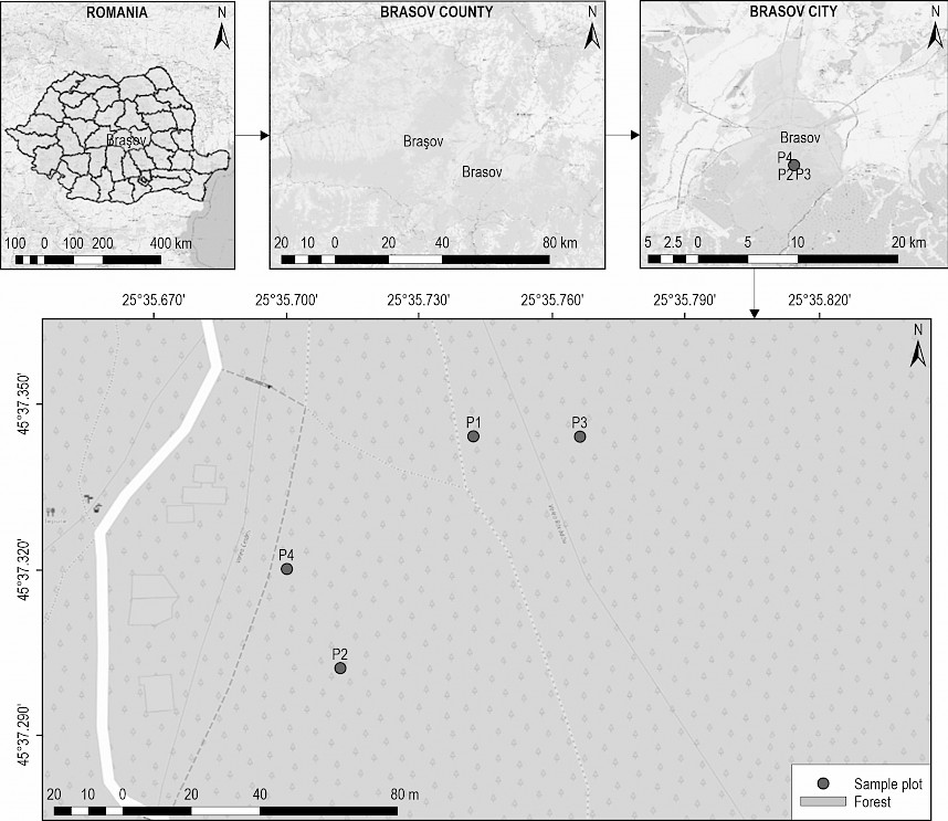
Fig. 1 Study area and location of sample plots designed using boundary shapefile of administrative areas of Romania and OSM Standard of QuickMapServices in QGIS 3.16.3 Hannover software

2.2 Machines Used and Condition of Skid Road Network in Study Area

In the area of study, the most common machines used for wood extraction were cable skidders, of which the domestic, Romanian-made brand was mainly used. These are typically light-weight machines (for instance: https://www.irum.ro/en/vehicle-listings/skidder-690-pe/), of up to 8 tons in unloaded state, that are used to transport the logs from the forest stand to the roadside landing. On the slopes, skid roads were developed some years ago for selective extractions. Over time, these roads have been subjected to a considerable amount of weathering and erosion, resulting in variations in the depth and shape across different sections of the skid road network.

2.3 Sample Plot Design and Field Measurements

Field data were collected in April 2022. On each of the four locations considered for the study, rectangular sample plots of approximately 2 by 10 m were delimited and geographically positioned by a handheld GPS receiver. In these plots, a sampling design was implemented (Fig. 2). In order to precisely geo-reference and calibrate the models when processing LiDAR data, ground control points (GCPs) are frequently used (Maté-González et al. 2022, Pixpro Team 2022); GCPs are markers on the target surface connected to a known accurate geographic coordinate point (Pixpro Team 2022). White plastic (waterproof) spheres of 20 cm in diameter were used in this study as GCPs. Each sphere was mounted on an impact-resistant plastic black stand inserted in the soil. To ensure a good contrast and an easy identification in the LiDAR-derived point clouds, the sides of each sphere were marked in advance with numbers from 1 to 10 and then the top center of each sphere was marked by a dot using a black permanent marker (Fig. 2). The perimeter of each plot was then marked by placing each GPC at intervals of 2 m from each other, based on measurements done by a tape so as to have a rectangular grid defined by distances of 2 m between the centers of the spheres. The GCPs were used to accurately geo-reference points on the scanned surface and to specify their coordinates (Talbot et al. 2018).

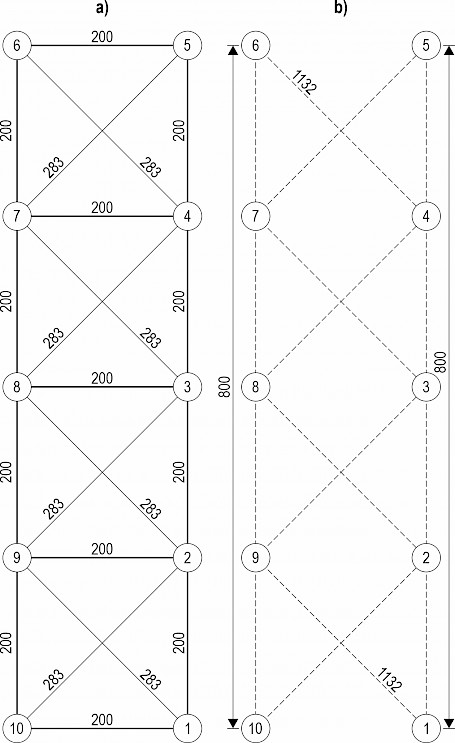
Fig. 2 Conceptual design of sample plots showing locations of ground control points (1–10): a – distances measured in field by a tape at plot level; b – distances computed in the office (each diagonal track, from 1–5 and from 6–10, had a length of ca. 1132 cm)

2.4 Manual Collection of Reference Data

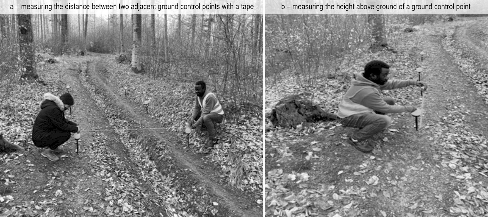
Fig. 3 Manual measurements between ground control points

Getting reference data involved manual measurements of actual distances between pairs of ground control points using a tape. The top marked centers of the spheres were used as starting and ending points of each measurement. All the possible distances between any two adjacent GCPs were measured by the tape to the nearest millimeter (Fig. 2a, Fig. 3a), and the distance results (21 in total for each plot) were noted in a field book. In the office phase of the study, the measurements taken manually by the tape were held as reference data and they were complemented by a set of 4 new measurements per plot consisting of the distances computed as the sums of the two diagonal tracks and the distances computed on the long plot sides (Fig. 2b). While the two schemes (Fig. 2) are only conceptual, the actual distances taken by the tape were noted and used to compute the distances (Fig. 3a).

2.5 Acquisition of LiDAR Data

Following the manual measurements, two LiDAR-based mobile devices – GeoSLAM Zeb-Revo (GeoSLAM Ltd: Ruddington, Nottinghamshire, UK 2017) and the iPhone 13 Pro Max (Apple Inc., Cupertino, CA, USA 2021) were used for scanning the sample plots. Two free apps were installed on the iPhone, namely SiteScape and 3DScanner App. The functionalities of SiteScape and 3DScanner apps enable them to create 3D scans of objects, which can be exported to most of the commonly used CAD software (Chambers et al. 2022, SiteScape Inc., ). The scanning procedure used for Zeb Revo was comparable to those used in previous studies (Gollob et al. 2020, 2021, Ryding et al. 2015). To scan each plot, the operator walked slowly following a route at about 1.5 m from the plot boundary, beginning and ending at the same point. This was done to make sure that the entire sample plot was covered by scanning, as well as to achieve a higher position accuracy, and lower drifts and scanner range noise. At the end of each scanning, the point cloud data were automatically processed by the device and saved onto a USB stick memory. For the mobile phone and used apps, three scanning resolutions were tested: low density, high density and medium density scans, respectively. The scanning was done by moving at walking speed along the axis of the plot while the LiDAR sensor collected the 3D measurement data. The point cloud data collected by the two LiDAR platforms were downloaded in a personal computer at the end of each day of measurement.

2.6 Processing of Lidar-Derived Data to Produce Raw Distance Data

Point cloud data processing was done in the free software program CloudCompare (version 2.12 beta; Girardeau-Montaut 2015) and aimed at extracting information on the distances between point-pairs in the three-dimensional space, having as a reference the distances collected manually. The point clouds were imported from the LiDAR scans in a LAZ file format (.laz) (Thomson 2018). After cleaning the clouds using the noise filter tool, the data were segmented using the interactive segmentation tool (Girardeau-Montaut 2015), exported, and saved in PLY MESH (.ply) file format (Thomson 2018). Using the point-picking tool (Girardeau-Montaut 2015), the distances between the point-pairs were measured (Fig. 4) and recorded in a Microsoft Excel® spreadsheet (Microsoft, ).

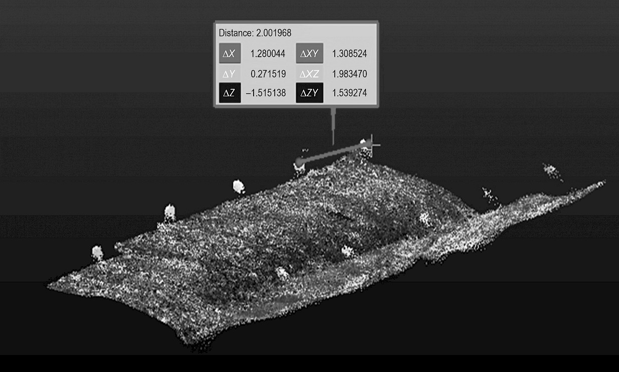
Fig. 4 Distance computation using point picking tool in CloudCompare

Ten measurements were taken for each point-pair. Although several scanning resolutions were tested, only the MD files were used for processing. The reason for this choice was that after a careful visual analysis of all the files, it was observed that the MD scans retained a very high quality.

2.7 Preparation of Raw Distance Data and Comparative Statistical Analyses

The ten LiDAR-based raw distance data taken between each two GCPs of each point cloud were included in a looped procedure for outlier detection with the aim of iteratively removing outlying data until reaching a stable dataset (i.e. without outliers) to be used for the calculation of the mean value. Outlier exclusion was implemented by the use of box-plot functionalities of Microsoft Excel®, and it produced the datasets used to compute the LiDAR-based distances. Following this procedure, the minimum number of values retained for mean calculation was five, but the dominant ones were between eight and ten. The mean values were rounded to the nearest millimeter, and they were used for pairwise comparison in a Microsoft Excel® spreadsheet aimed at identifying the agreement between the manual and LiDAR based methods. One manual and four LiDAR-derived datasets were used in the data analyses (Table 1).

Table 1 Description of datasets used in statistical data analyses

Variable	Dataset
RD	Manual reference data
SA1	Mean LiDAR-derived data based on 3D Scanner App. Scanning settings: normal, normal area, medium density. Export: medium density
SA2	Mean LiDAR-derived data based on 3D Scanner App. Scanning settings: advanced, low area, medium density. Export: medium density
SS	Mean LiDAR-derived data based on SiteScape. Scanning settings: maximum area, medium density. Export: medium density
ZR	Mean LiDAR-derived data based GeoSlam Zeb Revo. Scanning settings: as provided by device. Export: as provided by the dedicated software

Then, a Bland and Altman analysis was performed to assess the agreement between the scanned and manual reference data (Bland and Altman 1986 and 1999). This method involves plotting the means of each pair of measurements against the differences between them in a bi-dimensional space characterized by a 95% prediction interval bounded by the limits of agreement (LOA), which are computed based on the bias and the standard deviation in differences (Bland and Altman 1999, Giavarina 2015). For a confidence set at 95%, two standard deviations were considered (Bland and Altman 1999) to indicate a range where 95% of the differences between manual and LiDAR-based measurements are anticipated to fall. The extent of the potential sampling error can be estimated using the 95% confidence interval (CI) of agreement limits (Giavarina 2015). Accordingly, in this study the limits of agreement were calculated based on the mean of difference between the manual reference data and the LiDAR-derived data, by considering two standard deviations. Moreover, Breusch-Pagan and White tests were performed on the datasets to check if there was heteroscedasticity in data (Breusch-Pagan 1979, White 1980). Although the White test concept is similar to that of Breusch and Pagan, it is based on less solid premises on the shape that heteroscedasticity takes. As a result, the quadratic errors are regressed by the explanatory variables as well as by their squares and cross-products (Addinsoft 2022). Both Breusch-Pagan and White heteroscedasticity tests were used in this study to check whether the regression residuals had changing variance (Addinsoft 2022). Differences between manual and LiDAR-based estimates were checked by the commonly used error metrics, namely the mean absolute error (MAE), root mean square error (RMSE) and bias (BIAS). These were computed using as a reference the manual measurements with the aim to estimate the accuracy of the LiDAR-derived data. In this context, accuracy refers to how closely a measurement resembles its true value (Chen et al. 2018, Zhang and Goodchild 2002). The MAE is calculated as the average magnitude of positive differences between the predicted and actual observations over a sample, where each individual difference is given equal weight, while RMSE is the square root of the average of squared deviations between predicted and actual observations (Hodson 2022). The MAE has a lower sample variance compared with RMSE, indicating that it is the most robust choice, and unlike RMSE, it is an unambiguous and most natural measure of average error magnitude (Brassington 2017, Hodson 2022, Wilmott and Matsuura 2005). However, RMSE is considered to be the best metric for normally distributed errors, according to Chai and Draxler (2014). Although neither metric is always sufficient in practice, they are both useful when used properly (Hodson 2022). These error metrics may typically be used to evaluate the difference in paired values of the same variable when it is unclear which set of estimates is the most reliable (Wilmott and Matsuura 2005). As such, both MAE and RMSE were used to check the differences among the measurement techniques used in this study. Bias (BIAS) stands for the average value of differences. The estimated values of each LiDAR-derived data were pairwise compared with the manual reference data by the developing ordinary least square (OLS) linear regression and least square linear regression through origin models, which fitted the manually measured distances as dependent variables and the LiDAR-derived data as independent variables. This was done to estimate the relationship between the two datasets, to clarify if there was a close relationship, and to predict the value of the manual reference data at a certain value of the LiDAR-derived data (Bevans 2020). Then, the correlation between the manually measured and LiDAR-derived distance datasets was tested using Pearson (r) and Spearman (ρ) tests (Pearson 1895, Spearman 2010, Schober et al. 2018) to assess the strength of association between the two approaches to distance measurements. Typically, the Pearson coefficient (r) works with a linear relationship between the two variables, whereas the Spearman coefficient (ρ) works with relationships in which, as one variable increases, the other tends to either increase or decrease, but not necessarily in a monotonic way (Frost 2022, Ramzai 2020). The two correlation tests were conducted in order to reinforce and confirm the certainty of the association, while the regression analyses were run to infer the type of data dependence.

3. Results

3.1 Agreement in Measurement Data

As shown in Tab. 2, in general, heteroscedasticity was not present in the data, excepting SA2, by the Breusch-Pagan test. Moreover, most of the data indicated a significant agreement between the two methods (Fig. 5). In scientific terms, a significant agreement between the two methods suggests that they produce similar or consistent results. This indicates that the methods are reliable for further analysis or interpretation and can be used interchangeably or in conjunction with each other. The absence of heteroscedasticity further supports the reliability of the data, as it indicates that the variability of the measurements was relatively consistent across the range of values. Concerning the measured distances, approximately 81 observations (ca. 96.4%) of the 3D Scanner App at both scanning settings were found in between the limits of agreement (Fig. 5a, 5b). With SiteScape, 76 observations (ca. 90.5%) were found in between the limits of agreement (Fig. 5c), whereas with Zeb Revo, 82 observations (ca. 97.6%) were found within the limits of agreement (Fig. 5d). For the computed distances, 15 observations (93.8%) of all the LiDAR platforms were found within the limits of agreement.

Table 2 Results of heteroscedasticity tests (α=0.05)

Type of reference measurement data	Test	Statistic	LiDAR Dataset
						SA1	SA2	SS	ZR
Measured by tape	Breusch-Pagan	LM stat	1.989	4.750	0.082	3.008
				p-value	0.158	0.029	0.775	0.083
				F stat	1.988	4.914	0.080	3.046
				p-value	0.162	0.029	0.778	0.085
		White	LM stat	3.156	4.761	0.233	3.232
				p-value	0.206	0.093	0.890	0.199
				F stat	1.581	2.433	0.112	1.621
				p-value	0.212	0.094	0.894	0.204
Computed	Breusch-Pagan	LM stat	0.881	1.226	0.003	3.261
				p-value	0.348	0.268	0.959	0.071
				F stat	0.815	1.162	0.002	3.584
				p-value	0.382	0.299	0.962	0.079
		White	LM stat	3.171	1.384	0.281	4.683
				p-value	0.205	0.500	0.869	0.096
				F stat	1.606	0.616	0.116	2.689
				p-value	0.238	0.555	0.891	0.105
SA1 – 3D Scanner App based on normal, normal area, medium density scanning settings SA2 – 3D Scanner App based on advanced, low area, medium density scanning settings SS – SiteScape based on maximum area, medium density scanning settings ZR – Zeb Revo

Concerning the linear regression models for the measured distances, the two datasets were strongly linearly-related with 3D Scanner App at normal, normal area, medium density scanning settings, as shown by the coefficient of determination (R2=1.0, Fig. 6). Similarly with the 3D Scanner App at advanced, low area, medium density scanning setting, there was a significant agreement (R2=1.0, Fig. 6b) at least for the data range from 196.8 to 205.7 cm. However, the degree of discrepancy began to rise according to the range of the distances between 288.2 and 289.8 cm. With SiteScape and Zeb Revo, the two datasets were strongly linearly-related (R2=1.0, Fig. 6c, 6d). For all the models, the slope of least square linear regression through the origin was close to that of 1:1. Based on the linear regression models for the computed distances, there was a strong dependence relation between the distance estimations by the two methods (R2=1.0), and the slope of the regression line was very close to that of the perfect agreement (Fig. 6). The data clustered around the regression line indicates a very close relationship between the two methods of measurement. The correlation analysis indicated that there was a very strong positive association between the manually measured and LiDAR-based datasets. The tests results indicate that the Pearson's (r) and Spearman's correlation coefficient (ρ) were very close to 1 and they returned very significant figures (Table 3).

Table 3 Results of correlation analysis tests (α=0.05)

Type of reference measurement data	Test & diagnose	LiDAR Dataset
				SA1	SA2	SS	ZR
Measured by tape	Pearson (r)	0.9997	0.9993	0.9997	0.9996
		Diagnose	***	***	***	***
		Spearman (ρ)	0.9841	0.9608	0.9768	0.9813
		Diagnose	***	***	***	***
Computed	Pearson (r)	1.0000	0.9999	1.0000	0.9999
		Diagnose	***	***	***	***
		Spearman (ρ)	0.9647	0.9845	0.9618	0.9624
		Diagnose	***	***	***	***
SA1 – 3D Scanner App based on normal, normal area, medium density scanning settings SA2 – 3D Scanner App based on advanced, low area, medium density scanning settings SS – SiteScape based on maximum area, medium density scanning settings ZR – Zeb Revo

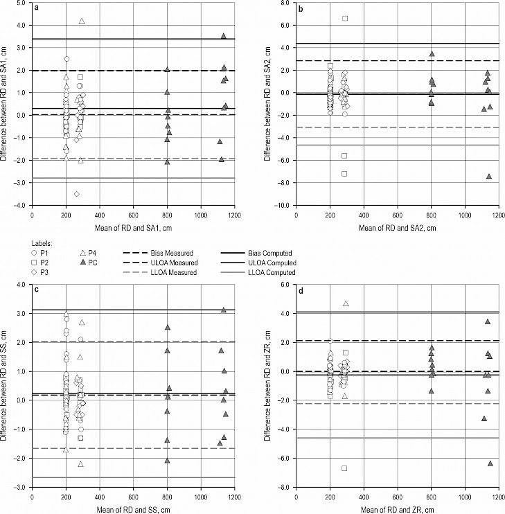
Fig. 5 Bland-Altman plots of measured (P1–P4) and computed (PC) data, showing bias (black lines), and lower and upper limits of agreement (gray lines): a – 3D Scanner App based on normal, normal area, medium density scanning settings (SA1); b – 3D Scanner App based on advanced, low area, medium density scanning settings (SA2); c – SiteScape based on maximum area, medium density scanning settings (SS); d – Zeb Revo. Note: RD stands for manual reference data

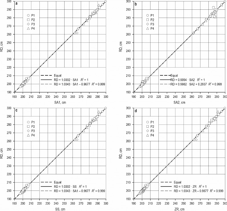
Fig. 6 Relation between manual reference (RD) and LiDAR-derived data for measured distances: a – 3D Scanner App based on normal, normal area, medium density scanning settings (SA1); b – 3D Scanner App based on advanced, low area, medium density scanning settings (SA2); c – SiteScape based on maximum area, medium density scanning settings (SS); d – Zeb Revo. Legend: P1–P4 stand for plot-level comparisons, dark grey dashed line stands for perfect agreement, black line stands for dependence relation between RD and LiDAR-derived data fitted by ordinary least square (OLS) linear regression, and light grey dashed line stands for dependence relation between two datasets fitted by least square linear regression through origin (RTO)

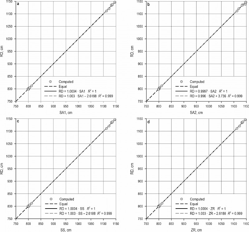
Fig. 7 Relation between manual reference data and LiDAR-derived data for computed distances: a – 3D Scanner App based on normal, normal area, medium density scanning settings (SA1); b – 3D Scanner App based on advanced, low area, medium density scanning settings (SA2); c – SiteScape based on maximum area, medium density scanning settings (SS); d – Zeb Revo. Legend: Computed stands for computed distances, dark grey dashed line stands for perfect agreement, black line stands for dependence relation between RD and LiDAR-derived data fitted by ordinary least square (OLS) linear regression, and light grey dashed line stands for dependence relation between two datasets fitted by least square linear regression through origin (RTO)

3.2 Error Metrics

For all the LiDAR datasets, the lowest error metrics were found when considering the measured distance dataset (Table 4). In this case, the bias of 3D Scanner App at normal, normal area medium density laser settings (BIAS=0.02 cm) was comparable to that of SiteScape based on maximum area, medium density scanning settings (BIAS=0.18 cm), since both returned positive values, indicating a slight underestimation. However, the bias of the 3D Scanner App at normal, normal area, medium density scanning settings was the lowest. Likewise, the bias of 3D Scanner App at advanced, low area, medium density scanning settings (BIAS=–0.12 cm) was similar to that of Zeb Revo (BIAS=–0.05 cm) because both returned slight overestimations. The MAE of 3D Scanner App at normal, normal area, medium density scanning settings (MAE=0.68 cm), SiteScape based on maximum area, medium density scanning settings (MAE=0.64 cm) and Zeb Revo (MAE=0.61 cm) were slightly lower than that of the 3D Scanner App at advanced, low area, medium density scanning settings (MAE=0.91 cm). Concerning the RMSE metric, the values for 3D Scanner App at normal, normal area medium density scanning settings (RMSE=0.99 cm) and SiteScape at maximum area, medium density scanning settings (RMSE=0.95 cm) were smaller than those of the 3D Scanner App at advanced, low area, medium density scanning settings (RMSE=1.51 cm) and Zeb Revo (RMSE=1.11 cm). For the computed distances, the bias metrics kept the same trend in over or underestimation, and values of all the metrics were higher in magnitude. The bias was found in between –0.24 and 0.30 cm, MAE between 1.13 and 1.56 cm, and RMSE between 1.45 and 2.23 cm.

Table 4 MAE, RMSE and BIAS metrics for the measured and computed distances

Type of reference measurement data	Error metric, cm	LiDAR Dataset
				SA1	SA2	SS	ZR
Measured by tape	BIAS	0.02381	–0.12381	0.17738	–0.05119
		MAE	0.68333	0.90714	0.64405	0.60833
		RMSE	0.98694	1.50910	0.94850	1.10577
Computed	BIAS	0.30000	–0.13750	0.23125	–0.24375
		MAE	1.27500	1.40000	1.13125	1.45625
		RMSE	1.55563	2.23327	1.44978	2.16348
SA1 – 3D Scanner App based on normal, normal area, medium density scanning settings SA2 – 3D Scanner App based on advanced, low area, medium density scanning settings SS – SiteScape based on maximum area, medium density scanning settings ZR – Zeb Revo

4. Discussion

The Bland-Altman analysis shows that the LiDAR-based data collected using two iPhone apps exhibited a high level of accuracy compared to the manual reference variant. The majority of distance measurements obtained from the apps fell within the limits of agreement ( and Puranik 2021), indicating a good fit to the manual reference. This finding suggests that the LiDAR-based data collected through the iPhone apps can be considered reliable and comparable to the manual reference variant. Analysis of the error metrics indicated that both SiteScape and 3D Scanner App can be used to accurately estimate soil disturbance in forest operations. Absolute errors for the two apps were all less than 2 cm, indicating a high accuracy of estimates. However, these findings, revealed that although the same LiDAR sensor was used for scanning, the outcomes from the two tested applications exhibited slight variations. This demonstrates how important the software component is when using the same hardware configuration (Gollob et al. 2021), as well as the limitations brought by the methods used to get the LiDAR-based, averaged distances.

In recent studies on LiDAR measurements, several factors have been identified that can contribute to over- and underestimations, including pulse density, pattern of scan (sensors), scan angles and relative noise (Fradette et al. 2019, Klaas-Witt and Emeis 2022). These factors can impact the accuracy of LiDAR measurements and should be taken into consideration when analysing the data (Fradette et al. 2019, Klaas-Witt and Emeis 2022). For instance, studies have shown that factors such as reduced relative noise and low density of the point clouds can cause underestimation, and vice versa (Borgogno Mondino et al. 2020, Gollob et al. 2021). Thus, the distance underestimation with SiteScape and 3D Scanner App based on normal area, medium density scanning settings, and the overestimation with 3D Scanner App based on advanced, low area, medium density scanning settings could probably be attributed to these factors. According to Borgogno Mondino et al. (2020), it can be expected that some of these inaccuracies also resulted from manual measurement errors. Distinguishing points reflected by the terrain from those reflected by other objects is one of the key challenges in modelling landscape-based LiDAR data (Koren et al. 2015). The presence of harvesting waste on the forest floor, stumps, or stones that have shifted due to skidding could also have an impact on the LiDAR-derived distance data (Salmivaara et al. 2021). However, it is suggested that prior to data collection, logging residues that were left on the ground should be cleared from the sampling area. According to Luetzenburg et al. (2021), some deviations may probably come from technical capabilities of the iPhone 13 Pro Max inertial measurement unit. In this study, however, some inaccuracy may also come from the difficulty in identifying and hitting the center of the spheres used as GCPs, although efforts were made to minimize this source of systematic error by taking ten measurements between each point-pair and averaging the results. However, some of the averaged values relied on only five measurements following the outlier exclusion loop.

Both the SiteScape and 3D Scanner App data, however, exhibited significant consistency with the manually measured distances, with low related MAEs and RMSEs. Similar results were reported by Mikita et al. (2022), who found that the best results were achieved with 3D Scanner App, with an RMSE of about 2 cm. Moreover, the Breusch-Pagan and White tests proved that there was no heteroscedasticity of residuals, excepting the 3D Scanner App based on the advanced low area, medium density scanning settings by Breusch-Pagan test (p=0.029). Ordinary least square (OLS) and regression through origin (RTO) were used in conjunction with heteroskedasticity tests, because they provide efficient and unbiased estimates of the variance of errors in the presence of homoskedasticity (Weerahandi 1995). The developed regression models confirmed the linear dependence relationship between the manual and the LiDAR-derived data. In a perfect linear match, the relationship between LiDAR-derived measurements and manual reference measurements should be deterministic. This means that the value of LiDAR-derived measurements should be equal to the manual reference measurements. In other words, when the manual reference data has a zero value, the expectation is that the LiDAR data should also have a zero value. This deterministic relationship implies a direct and precise correspondence (Hintze 2007) between the two measurement methods. For the ordinary least square linear regression models, the intercepts had values in the range of –2.6 to 3.7 cm, but most of them were found in lower ranges which, along with slopes close to 1 in all cases, confirmed the closeness to linear dependence relationships. Therefore, no important difference was found between the two methods, which confirms the accuracy of LiDAR-derived data.

Even though the findings of this study are particular to the research area, they are generally consistent with prior findings in terms of distance measurement (e.g. Mikita et al. 2022), and they offer some general advice for future soil mapping. In spite of the high accuracy and agreement of the low-cost LiDAR technology, this study is limited by the small sample size since it covered only four rectangular plots of approximately 20 m2 each. To mitigate this limitation and increase the likelihood that they are representative of the entire area of interest, the four sample plots were selected randomly from the larger forest area. The benefits of using random sampling include increased representativeness, reduced bias, increased precision, improved generalizability, and increased reliability of these findings (Feldman 2024). Besides, the plots were selected to represent the variations in topography and soil disturbance in the study area. Additionally, the sampling design of this study prevented the examination of the spatial relationships at distances higher than 12 m. The limitations of this study highlight the necessity of sampling designs that enable closer-range observations, if the researcher wishes to collect very accurate data and make use of the results in operational settings (Mauro et al. 2017). Based on our field experience, future options for operational 3D mapping of forest soil disturbance that seek to evaluate the accuracy of the LiDAR platforms should include or complement the field data collection in larger plots or the use of a plot shape made up of clusters of subplots. Clusters of observations might be obtained using such designs, which would improve sample designs that take into account spatial correlation of errors (Mauro et al. 2017, Zimmerman 2006). The results also imply that larger samples are needed to give a more robust assessment of soil disturbance. In several cases, the actual surface affected by the forest operations along skid trails may be considerably wider and typically longer (Ampoorter et al. 2010, Kore et al. 2015, Mohieddinne et al. 2022). As a result, the applicability of the low-cost LiDAR technology should be tested by considering both, a wider scanning area and longer plots. In this regard, the relative short scanning range of the iPhone 13 Pro max is likely to limit its use (Luetzenburg et al. 2021).

One should also keep in mind that the accuracy assessment was based on comparing distances derived from LiDAR scanning with those measured manually. None of these methods is errorless, since some deviation could be specific to manual measurements as opposed to the ground truth values, while the LiDAR-based data was statistically inferred in this study based on measurements done by taking the starting and ending points in the point clouds as close as possible to the centers of the GCPs seen in the data. Accordingly, there was less control over the starting and ending LiDAR points in actually hitting the center of the GCPs. Since this study was based on distance measurement and comparison, it remains to be researched how the texture and roughness of the soil over the skid trails could affect the agreement and accuracy of more detailed measurements, by finding a suitable way to measure the reference data in more detail. To conclude, the concept of this study relies on the logic, that if the distances were in agreement and accurate, then the whole point cloud would be characterized by the same degree of agreement and accuracy. To our knowledge, on the other hand, there are no formalized limits of accuracy when estimating the soil disturbance by compaction. Indeed, the practice in assessing this type of disturbance is frequently based on rut measurements and may use depth categories with steps of 10 cm. Under this point of view, there is a high potential of LiDAR-based methods in providing data at an improved degree of accuracy, as shown by this study, which may include a better microstructure mapping over the trafficked soil surface as compared to the current estimation practice.

Notwithstanding this, it is very easy and convenient to use the iPhone 13 Pro Max for scanning due to its small size. Besides, there is no need for prior preparation to use the LiDAR scanner and this will facilitate direct and prompt data collection in the future. As a result, researchers, forest owners and managers will be able to monitor soil disturbance and environmental change. In addition, the data can be shared between platforms without the need for global geo-referencing, by exporting the collected point clouds or data meshes in a variety of formats (Luetzenburg et al. 2021, Mikita et al. 2022). Future developments in low-cost technology will probably continue to advance so as to provide greater autonomy and range, as well as better, more affordable, and more precise sensors. As a result, it is expected that high resolution 3D models of forest soils created by affordable LiDAR technology would be used in a growing number of forestry applications in the near future.

5. Conclusions

For small study plots, the centimeter-level scanning accuracy of the iPhone 13 Pro Max and the integrated low-cost LiDAR technology (MAE=0.64–1.40) are similar to those of professional platforms (MAE=0.61–1.46), which may satisfy the general requirements of small-scale high-quality 3D soil mapping. For estimating and mapping soil disturbance in forest operations, the iPhone's LiDAR scanner offers an effective, trustworthy, affordable, and significantly less labor-intensive alternative. These findings might provide the basis for further studies on the applicability of this low-cost LiDAR technology to larger sample sizes and different operating conditions. By conducting further studies on the effectiveness of this technology, researchers can provide a more comprehensive understanding of its potential for various applications, while also addressing any potential limitations or challenges that may arise. This approach could enable the development of new and improved techniques for low-cost mobile LiDAR data collection, analysis, and interpretation while creating opportunities for advancements in various fields such as forestry and agriculture.

Acknowledgements

The authors would like to thank to Jenny Magaly Morocho Toaza for her help in the field data collection stage. The authors would like to thank to the Department of Forest Engineering, Forest Management Planning, and Terrestrial Measurements, Faculty of Silviculture and Forest Engineering, Transilvania University of Brasov, for providing the equipment needed for this study. Some activities in this study were funded by the inter-institutional agreement between Transilvania University of Brasov and Mediterranean University of Reggio Calabria.

Funding

This work was supported by the Transilvania University of Brasov – grant »Proiectul Meu de Diploma 2022«, which supported the purchase of some of the equipment used in the field data collection. Some of the activities of this study were supported by two grants of the Romanian Ministry of Education and Research, CNCS – UEFISCDI, project number PN-IV-P8-8.1-PRE-HE-ORG-2023-0141, and project number PN-IV-P8-8.1-PRE-HE-ORG-2024-0186, within PNCDI IV.

6. References

Addinsoft, 2022: Heteroscedasticity Tests. Available online: https://www.xlstat.com/en/solutions/features/heteroscedasticity-tests (Accessed December 30, 2022)

Ampoorter, E., Goris, R., Cornelis, W.M., Verheyen, K., 2007: Impact of mechanized logging on compaction status of sandy forest soils. For. Ecol. Manage. 241(1–3): 162–174. https://doi.org/10.1016/j.foreco.2007.01.019

Ampoorter, E., Van Nevel, L., De Vos, B., Hermy, M., Verheyen, K., 2010: Assessing the effects of initial soil characteristics, machine mass and traffic intensity on forest soil compaction. For. Ecol. Manage. 260(10): 1664–1676. https://doi.org/10.1016/j.foreco.2010.08.002

Ampoorter E., de Schrijver, A., van Nevel, L., Hermy M., Verheyen K., 2012: Impact of mechanized harvesting on compaction of sandy and clayey forest soils: results of a meta-analysis. Ann. For. Sci. 69: 533–542. https://doi.org/10.1007/s13595-012-0199-y

Bevans, R., 2020: Simple linear regression. An easy introduction & examples. Available online: https://www.scribbr.com/statistics/simple-linear-regression/

Bland, J.M., Altman, D.G., 1986: Statistical methods for assessing agreement between two methods of clinical measurement. Lancet 327(8476): 307–310. https://doi.org/10.1016/S0140-6736(86)90837-8

Bland, J.M., Altman, D.G., 1999: Measuring agreement in method comparison studies. Stat. Methods Med. Res. 8(2): 135–160. https://doi.org/10.1177/096228029900800204

Borgogno Mondino, E., Fissore, V., Falkowski, M.J., Palik, B., 2020: How far can we trust forestry estimates from low-density LiDAR acquisitions. The Cutfoot Sioux experimental forest (MN, USA) case study. Int. J. Remote Sens. 41(12): 4549–4567. https://doi.org/10.1080/01431161.2020.1723173

Borz, S.A., Crăciun, B.C., Marcu, M.V., Iordache, E., Proto, A.R., 2023: Could timber winching operations be cleaner? An evaluation of two options in terms of residual stand damage, soil disturbance and operational efficiency. Eur. J. For. Res. 142(3): 1–17. https://doi.org/10.1007/s10342-023-01536-1

Borz, S.A., Ignea, G., Popa, B., Spârchez, G., Iordache, E., 2015: Estimating time consumption and productivity of roundwood skidding in group shelterwood system–a case study in a broadleaved mixed stand located in reduced accessibility conditions. Croat. J. For. Eng. 36(1): 137–146.

Brassington, G., 2017: Mean absolute error and root mean square error: which is the better metric for assessing model performance? In EGU General Assembly Conference Abstracts, 3574 p

Breusch, T.S., Pagan, A.R., 1979: A simple test for heteroscedasticity and random coefficient variation. Econometrica 47(5): 1287–1294. https://doi.org/10.2307/1911963

Chai, T., Draxler, R.R., 2014: Root mean square error (RMSE) or mean absolute error (MAE)? – Arguments against avoiding RMSE in the literature. Geosci. Model Dev. 7(3): 1247–1250. https://doi.org/10.5194/gmd-7-1247-2014

Chen, J., Mora, O.E., Clarke, K.C., 2018: Assessing the accuracy and precision of imperfect point clouds for 3D indoor mapping and modeling. ISPRS Ann. Photogramm. Remote Sens. Spatial Inf. Sci. (IV-4/W6): 3–10. https://doi.org/10.5194/isprs-annals-IV-4-W6-3-2018

Dudáková, Z., Allman, M., Merganič, J., Merganičová, K., 2020: Machinery-induced damage to soil and remaining forest stands – Case study from Slovakia. Forests 11(12): 1289. https://doi.org/10.3390/f11121289

Di Stefano, F., Chiappini, S., Gorreja, A., Balestra, M., Pierdicca, R., 2021: Mobile 3D scan LiDAR: a literature review. Geomatics Nat. Hazards Risk 12(1): 2387–2429. https://doi.org/10.1080/19475705

Duţă, C.I., Sălăjan, A., Borz, S.A., 2018: Estimating current state of soil erosion induced by skid trails geometry in mountainous conditions. Environ. Eng. Manag. J. 17(3): 697–704.

Feldman, K., 2024: Random sampling: key to reducing bias and increasing accuracy. Available online: https://www.isixsigma.com/dictionary/random-sampling/ (Accessed March 7, 2024)

Fradette, M.S., Leboeuf, A., Riopel, M., Bégin, J., 2019: Method to reduce the bias on digital terrain model and canopy height model from LiDAR data. Remote Sens. 11(7): 863. https://doi.org/10.3390/rs11070863

Frey, B., Kremer, J., Rüdt, A., Sciacca, S., Matthies, D., Lüscher, P., 2009: Compaction of forest soils with heavy logging machinery affects soil bacterial community structure. Eur. J. Soil Biol. 45(4): 312–320. https://doi.org/10.1016/j.ejsobi.2009.05.006

Frost, J., 2022: Spearman's correlation explained. Available online: https://statisticsbyjim.com/basics/spearmans-correlation/ (Accessed December 30, 2022)

Gambella, F., Sistu, L., Piccirilli, D., Corposanto, S., Caria, M., Arcangeletti, E., Proto, A.R., Chessa, G., Pazzona, A., 2016: Forest and UAV: A bibliometric review. Contemp. Eng. Sci. 9(28): 1359–1370. http://dx.doi.org/10.12988/ces.2016.68130

GeoSLAM Ltd. Ruddington, Nottinghamshire, 2017: ZEB-REVO user manual v3.0.0. Available online: https://download.geoslam.com (Accessed October 3, 2022)

Giavarina, D., 2015: Understanding Bland Altman analysis. Biochem. Medica. 25(2): 141–151. https://doi.org/10.11613/BM.2015.015

Girardeau-Montaut, D., 2015: CloudCompare: 3D point cloud and mesh processing software. Open Source Project, 197.

Gollob, C., Ritter, T., Kraßnitzer, R., Tockner, A., Nothdurft, A., 2021: Measurement of forest inventory parameters with Apple iPad Pro and integrated LiDAR Technology. Remote Sens. 13(16): 3129. https://doi.org/10.3390/rs13163129

Guimarães, N., Pádua, L., Marques, P., Silva, N., Peres, E., Sousa, J.J., 2020: Forestry Remote Sensing from Unmanned Aerial Vehicles: A Review Focusing on the Data, Processing and Potentialities. Remote Sens. 12(6): 1046. https://doi.org/10.3390/rs12061046

Hintze, J.L., 2007: Correspondence analysis. NCSS. Available online: https://www.ncss.com/wp-content/themes/ncss/pdf/Procedures/NCSS/Correspondence_Analysis.pdf (Accessed March 7, 2024)

Hodson, T.O., 2022: Root-mean-square error (RMSE) or mean absolute error (MAE): when to use them or not. Geosci. Model Dev. 15(14): 5481–5487. https://doi.org/10.5194/gmd-15-5481-2022

Hullette, T., Ghadge, P., Ali, A., 2023: The best 3D scanner apps of 2023 (iPhone & Android). Available online at: https://all3dp.com/2/best-3d-scanner-app-iphone-android-photogrammetry/ (Accessed March 7, 2024)

iPhone 13 Pro and iPhone 13 Pro Max-Apple, 2022: Available online: https://www.apple.com/iphone-13-pro/ (Accessed February 3, 2022)

Karun, K.M., Puranik, A., 2021: BA plot: An R function for Bland-Altman analysis. Clin. Epidemiol. Glob. Health 12: 100831. https://doi.org/10.1016/j.cegh.2021.100831

Klaas-Witt, T., Emeis, S., 2022: The five main influencing factors for lidar errors in complex terrain. Wind Energy Sci. 7(1): 413–431. https://doi.org/10.5194/wes-7-413-2022

Koreň, M., Slančík, M., Suchomel, J., Dubina, J., 2015: Use of terrestrial laser scanning to evaluate the spatial distribution of soil disturbance by skidding operations. iForest 8(3): 386–393. https://doi.org/10.3832/ifor1165-007

Latterini, F., Venanzi, R., Papa I., Đuka, A., Picchio, R., 2024: A Meta-Analysis to Evaluate the Reliability of Depth-to-Water Maps in Predicting Areas Particularly Sensitive to Machinery-Induced Soil Disturbance. Croat. J. For. Eng. 45(2):433–444. https://doi.org/10.5552/crojfe.2024.2559

Latterini, F., Dyderski, M.K., Horodecki, P., Rawlik, M., Stefanoni, W., Högbom, L., Venanzi, R., Picchio, R., Jagodziński, A.M., 2024: A Meta-analysis of the effects of ground-based extraction technologies on fine roots in forest soils. Land Degrad. Dev. 35(1): 9–21. https://doi.org/10.1002/ldr.4902

Luetzenburg, G., Kroon, A., Bjørk, A.A., 2021: Evaluation of the Apple iPhone 12 Pro LiDAR for an application in geosciences. Sci. Rep. 11(1): 1–9. https://doi.org/10.1038/s41598-021-01763-9

Macrì, G., Zimbalatti, G., Russo, D., Proto, A.R., 2016: Measuring the mobility parameters of tree-length forwarding systems using gps technology in the italian apennines. Agron. Res. 14(3): 836–845.

Marchi, E., Chung, W., Visser, R., Abbas, D., Nordfjell, T., Mederski, P.S., McEwan, A., Brink, M., Laschi, A., 2018: Sustainable Forest Operations (SFO): A new paradigm in a changing world and climate. Sci. Total Environ. 634: 1385–1397. https://doi.org/10.1016/j.scitotenv.2018.04.084

Marchi, E., Picchio, R., Spinelli, R., Verani, S., Venanzi, R., Certini, G., 2014: Environmental impact assessment of different logging methods in pine forests thinning. Ecol. Eng. 70: 429–436. https://doi.org/10.1016/j.ecoleng.2014.06.019

Maté-González, M.Á., Di Pietra, V., Piras, M., 2022: Evaluation of different LiDAR technologies for the documentation of forgotten cultural heritage under forest environments. Sensors 22(16): 6314. https://doi.org/10.3390/s22166314

Mauro, F., Monleon, V.J., Temesgen, H., Ruiz, L.A., 2017: Analysis of spatial correlation in predictive models of forest variables that use LiDAR auxiliary information. Can. J. For. Res. 47(6): 788–799. https://doi.org/10.1139/cjfr-2016-0296

Mikita, T., Krausková, D., Hrůza, P., Cibulka, M., Patočka, Z., 2022: Forest road wearing course damage assessment possibilities with different types of laser scanning methods including new iPhone LiDAR scanning apps. Forests 13(11): 1763. https://doi.org/10.3390/f13111763

Mohieddinne, H., Brasseur, B., Gallet-Moron, E., Lenoir, J., Spicher, F., Kobaissi, A., Horen, H., 2022: Assessment of soil compaction and rutting in managed forests through an airborne LiDAR technique. Land Degrad Dev. 34(5): 1558–1569. https://doi.org/10.1002/ldr.4553

Nugent, C., Kanali, C., Owende, P.M., Nieuwenhuis, M., Ward, S., 2003: Characteristic site disturbance due to harvesting and extraction machinery traffic on sensitive forest sites with peat soils. For. Ecol. Manage., 180(1–3): 85–98. https://doi.org/10.1016/S0378-1127(02)00628-X

Obabire Akinleye, A., Agboola, J.O., Ajao Isaac, O., Adegbilero-Iwari Oluwaseun, E., 2020: Comparison of different tests for detecting heteroscedasticity in datasets. Ann. Comput. Sci. 18(2): 78–85.

Papandrea, S.F., Stoilov, S., Angelov, G., Panicharova, T., Mederski, P.S., Proto A.R., 2023: Modeling productivity and estimating costs of processor tower yarder in shelterwood cutting of pine stand. Forests 14(2): 195. https://doi.org/10.3390/f14020195

Picchio, R., Mederski, P.S., Tavankar, F., 2020: How and how much, do harvesting activities affect forest soil, regeneration and stands? Curr. For. Rep. 6(2): 115–128. https://doi.org/10.1007/s40725-020-00113-8

Pixpro Team, 2022: Ground control points. The cornerstone of accuracy. Available online: https://www.pix-pro.com/blog/post/ground-control-points-accuracy (Accessed December 9, 2022)

Proto, A.R., Macrì, G., Sorgonà, A., Zimbalatti, G., 2016: Impact of skidding operations on soil physical properties in Southern Italy. Cont. Eng. Sc. 9(23): 1105–1112. https://doi.org/10.12988/ces.2016.68132

Ramzai, J., 2020: Clearly explained: Pearson V/S Spearman correlation coefficient. Available online: https://towardsdatascience.com/clearly-explained-pearson-v-s-spearman-correlation-coefficient-ada2f473b8 (Accessed December 30, 2022)

Ryding J., Williams E., Smith M.J., Eichhorn M.P., 2015: Assessing handheld mobile laser scanners for forest surveys. Remote Sens. 7(1): 1095–1111. https://doi.org/10.3390/rs70101095

Salmivaara, A., Miettinen, M., Finér, L., Launiainen, S., Korpunen, H., Tuominen, S., Heikkonen, J., Nevalainen, P., Sirén, M., Ala-Ilomäki, J., Uusitalo, J., 2018: Wheel Rut Measurements by Forest Machine-Mounted LiDAR Sensors-Accuracy and Potential for Operational Applications? Int. J. For. Eng. 29(1): 41–52. https://doi.org/10.1080/14942119.2018.1419677

Schack-Kirchner, H., Fenner, P.T., Hildebrand, E.E., 2007: Different responses in bulk density and saturated hydraulic conductivity to soil deformation by logging machinery on a Ferralsol under native forest. Soil Use Manage. 23(3): 286–293. https://doi.org/10.1111/j.1475-2743.2007.00096.x

Schober, P., Boer, C., Schwarte, L.A., 2018: Correlation coefficients: Appropriate use and interpretation. Anesth. Analg. 126(5): 1763–1768. https://doi.org//10.1213/ANE.0000000000002864

Spearman, C., 2010: The proof and measurement of association between two things. Int. J. Epidemiol. 39(5): 1137–1150. https://doi.org/10.1093/ije/dyq191

Stoilov, S., Proto, A.R., Angelov, G., Papandrea, S.F., Borz, S.A., 2021: Evaluation of salvage logging productivity and costs in the sensitive forests of Bulgaria. Forests 12(3): 309. https://doi.org/10.3390/f12030309

Talbot, B., Pierzchała, M., Astrup, R., 2017: Applications of remote and proximal sensing for improved precision in forest operations. Croat. J. For. Eng. 38(2): 327–336.

Talbot, B., Astrup, R., 2021: A review of sensors, sensor-platforms and methods used in 3D modelling of soil displacement after timber harvesting. Croat. J. For. Eng. 42(1): 149–164. https://doi.org/10.5552/crojfe.2021.837

Talbot, B., Rahlf, J., Astrup, R., 2018: An operational UAV-based approach for stand-level assessment of soil disturbance after forest harvesting. Scand. J. For. Res. 33(4): 387–396. https://doi.org/10.1080/02827581.2017.1418421

Thomson, C., 2018: Common 3D point cloud file formats & solving interoperability issues. Available online: https://info.vercator.com/blog/what-are-the-most-common-3d-point-cloud-file-formats-and-how-to-solve-interoperability-issues (Accessed December 11, 2022)

Weerahandi, S., 1995: ANOVA under unequal error variances. Biometrics 51(2): 589–599. https://doi.org/10.2307/2532947

White, H., 1980: A heteroskedasticity-consistent covariance matrix estimator and a direct test for heteroskedasticity. Econometrica 48(4): 817–838. https://doi.org/10.2307/1912934

Williamson, J.R., Neilsen, W.A., 2000: The influence of forest site on rate and extent of soil compaction and profile disturbance of skid trails during ground-based harvesting. Can. J. For. Res. 30(8): 1196–1205. https://doi.org/10.1139/x00-041

Wilmott, C.J., Matsuura, K., 2005: Advantages of the mean absolute error (MAE) over the root mean squared error (RMSE) in assessing the average model performance. Clim. Res. 30(1): 79–82. https://doi.org/10.3354/cr030079

ZEB Revo RT-GeoSLAM, 2022: Available online: https://geoslam.com/solutions/zeb-revo-rt/ (Accessed April 1, 2022)

Zhang, J., Goodchild, M.F., 2002: Uncertainty in geographical information (1st ed.). CRC Press. https://doi.org/10.1201/b12624

Zimmerman, D.L., 2006: Optimal network design for spatial prediction, covariance parameter estimation, and empirical prediction. Environmetrics 17(6): 635–652. https://doi.org/10.1002/env.769

© 2025 by the authors. Submitted for possible open access publication under the
terms and conditions of the Creative Commons Attribution (CC BY) license (http://creativecommons.org/licenses/by/4.0/).

Authors' addresses:

Gabriel Osei Forkuo, MSc

e-mail: gabriel.forkuo@unitbv.ro

Prof. Stelian Alexandru Borz, PhD

e-mail: stelian.borz@unitbv.ro

Transilvania University of Braşov

Faculty of Silviculture and Engineering

Department of Forest Engineering

Forest Management Planning and Terrestrial Measurements

Şirul Beethoven No. 1

500 123 Braşov

ROMANIA

Assoc. prof. Andrea Rosario Proto, PhD *

e-mail: andrea.proto@unirc.it

University Mediterranea of Reggio Calabria

Department of Agraria

Feo di Vito 89122

Reggio Calabria

ITALY

* Corresponding author

Received: June 18, 2024

Accepted: November 26, 2024

Original scientific paper

16

Download PDF