Estimation of Road Depression Depth Using Airborne Laser Scanned Data

Direct quality estimation studies of forest roads using remote sensed data are still rare. Research focussing on deriving indirect factors about road quality such as wetness or soil bearing capacities are prone to uncertainty of estimates. Altough processes of direct 3D roadsurface measurements and assesements exist, those systems mostly rely on ground-based collection methods, which are laborious and expensive for big forest road networks. Because of the increased quality of airborne laser scanned data (ALS) over the last decades, it was researched how this development may be used for forest road infrastructure assesement. The present study uses ALS data to estimate the occurrence of road damage in the form of concave depression. Maximum damage depth measurents were collected in a test area near Ilomantsi (Finland) and used to fit a linear mixed effect model to a subset of variables derived from ALS data as fixed factor and location as random factor. Simultaniously, depth measurements were carried out in a digital terrain model and compared to the real depth values to gain insight into maximum reachable accuracies. It was detected that ALS data tend to underestimate road damage depressions, limiting results in follow up models. Our results also indicate that road location could explain up to 30% of the variablity in our models. In the most optimal case, a linear mixed effect model could achieve an R2 of 0.87 with and 0.66 without the random factor having a residual mean standard error (RSME) of 1.9 to 2.7 cm on unvegetated forest roads. The best performing model determined in our study using ALS derived variables reached an R2 of 0.58 and 0.44 with an RSME of 1.8 to 2.4 cm. The work conducted gave insight into the culprits and limits of road depression depth estimates using ALS data. Future research should be conducted to change the scope of the analysis to an evaluation of bigger road segments and to investigate how road location could be utilized to achieve results with better accuracies.

Estimation of Road Depression Depth Using Airborne Laser Scanned Data

Maik Grabow, Timo Tokola, Vesa Leppänen

https://doi.org/10.5552/crojfe.2025.2487

Abstract

Direct quality estimation studies of forest roads using remote sensed data are still rare. Research focussing on deriving indirect factors about road quality such as wetness or soil bearing capacities are prone to uncertainty of estimates. Altough processes of direct 3D roadsurface measurements and assesements exist, those systems mostly rely on ground-based collection methods, which are laborious and expensive for big forest road networks. Because of the increased quality of airborne laser scanned data (ALS) over the last decades, it was researched how this development may be used for forest road infrastructure assesement. The present study uses ALS data to estimate the occurrence of road damage in the form of concave depression. Maximum damage depth measurents were collected in a test area near Ilomantsi (Finland) and used to fit a linear mixed effect model to a subset of variables derived from ALS data as fixed factor and location as random factor. Simultaniously, depth measurements were carried out in a digital terrain model and compared to the real depth values to gain insight into maximum reachable accuracies. It was detected that ALS data tend to underestimate road damage depressions, limiting results in follow up models. Our results also indicate that road location could explain up to 30% of the variablity in our models. In the most optimal case, a linear mixed effect model could achieve an R2 of 0.87 with and 0.66 without the random factor having a residual mean standard error (RSME) of 1.9 to 2.7 cm on unvegetated forest roads. The best performing model determined in our study using ALS derived variables reached an R2 of 0.58 and 0.44 with an RSME of 1.8 to 2.4 cm. The work conducted gave insight into the culprits and limits of road depression depth estimates using ALS data. Future research should be conducted to change the scope of the analysis to an evaluation of bigger road segments and to investigate how road location could be utilized to achieve results with better accuracies.

Keywords: forest roads, damage detection, road infrastructure, road maintenance

1. Introduction

Forest roads are an integral part of the forest infrastructure in Finland and a large part of the Finnish road network consists of private roads (350,000 km) that are used to access forest areas (Korpilahti 2008). Unpaved forest roads are used for wood transportation, to facilitate machine access, for travel to permanent settlements or as access for firefighters. It is important that these roads are maintained in good condition. Given the rise in vehicle weights in recent decades, many of the roads that were constructed between 1960 and 1995 are not suitable to carry heavy traffic (Korpilahti 2008). Continuous road quality monitoring and maintenance can help to compensate for that drawback and aids to maintain the road network.

Road condition monitoring is a crucial part of road maintenance. In particular, assessment as to where the damage has occurred and the intensity of such damage. When maintenance needs are well characterised, organised planning and the required resources can be allocated to maintenance operations. Studies on forest road trafficability, for example, manual measurements or capture of data via ground–applied mobile devices (e.g. Dapeng and Li 2021, Javad Heidari et al. 2022, Hoseini et al. 2024), are laborious as the data must be collected directly from the field. Despite the rapid change in the conditions of gravel roads (Selim and Skorseth 2000), repeated observations of more than a subset of selected forest roads may not be economically feasible when the labour requirements to capture the data are considered. Furthermore, techniques, such as the recording of vibrations using an accelerometer, must be taken in a standardised way that considers all influencing factors to ensure consistent results. These factors can include driving speed, vehicle suspension, arrangement of the measurement device sensors, as well as the sensor types (Edvardsson et al. 2015).

Other studies have linked forest trafficability to secondary factors, such as wetness (Uusitalo et al. 2020, Salmivaara 2020, Waga et al. 2020) or the soil bearing capacity (Vuorimies et al. 2015). This information could be captured by remotely sensed platforms or collected through field data. The drawback to this approach is that, while many studies have estimated the unfavourable conditions of the roads, they do not quantify the extent of the damage. Damage could also be linked to other factors, such as poor road management, unsuitable paving material, variation in the local construction material or intensity of the passing traffic. Also, some studies report relatively low accuracy when single datasets are used, which strengthens the need for further integration of dynamic datasets, such as seasonal wetness variation (Vuorimies et al. 2015, Hoffmann et al. 2022) or road condition class (e.g. Waga 2021).

Taking into account the drawbacks of the above methods, the use of remote sensed data and direct estimation processes seem to be an alternative to indirect estimation approaches. Studies using satellite imagery or data based on three-dimensional data, such as airborne (ALS) or terresrical laser scanning (TLS), achieved satisfactory results in estimating road conditions. A recent study from Greece (Kelesakis et al. 2024) has proposed a framework for estimating different road paramters including road quality, based on multispectral satellite imagery using various machine learning classification approaches. Another study evaluates the condition of unpaved roads in Tanzania based on satelite imagery derived statistical measures (Workman et al. 2023).

Studies from Finland and the Czech Republic indicate that ALS as well as TLS data can be used to estimate the condition of the road surface (Kiss et al. 2016, Hrůza et. al. 2018).

However, most methods estimating road quality expressed as quality categories, based their estimates on the damage classification system of the respective country. As these systems differ in their defintion of road damages as well as the amount of damage categories, it is hard to compare these measures between each other. An alternative approach to this challenge would be the estimation of a continuos direct measure describing road quality, which could be universally applicable while avoiding loosing information trough classification.

Therefore the aim of this study is to estimate the depth of road depressions (as a possible indicator of road quality) using an airborne lidar-based prediction methodology to determine gravel-road surface damage on roads with varying surface geometries. Our underlying assumption is that the difference in the damaged road surface from its optimal shape could lead to insights as to where the damage occurred and its intensity. An experiment was conducted to investigate how airborne laser scanning (ALS) data could be used to reliably predict road quality in the form of a continuous measure.

2. Materials and Methods

Field data were collected from a forest road network located between Tuupovaara and Ilomantsi (N 62° 36' 53, E 30° 40' 41 [UTM WGS84]) in North Karelia (Finland). The research area is characterised by intense forestry use and a relatively sparse population density. The annual mean temperature ranges from 3 to 4°C with mean annual precipitation from 650 to 700 mm. (Ilmatieteenlaitos 2023). The landscape mostly consists of flat to moderate hilly areas, with about 58 m in difference between the lowest and highest sample points. The most common soil types in the study area are sand moraines, peatland bedrock and mixed soils.

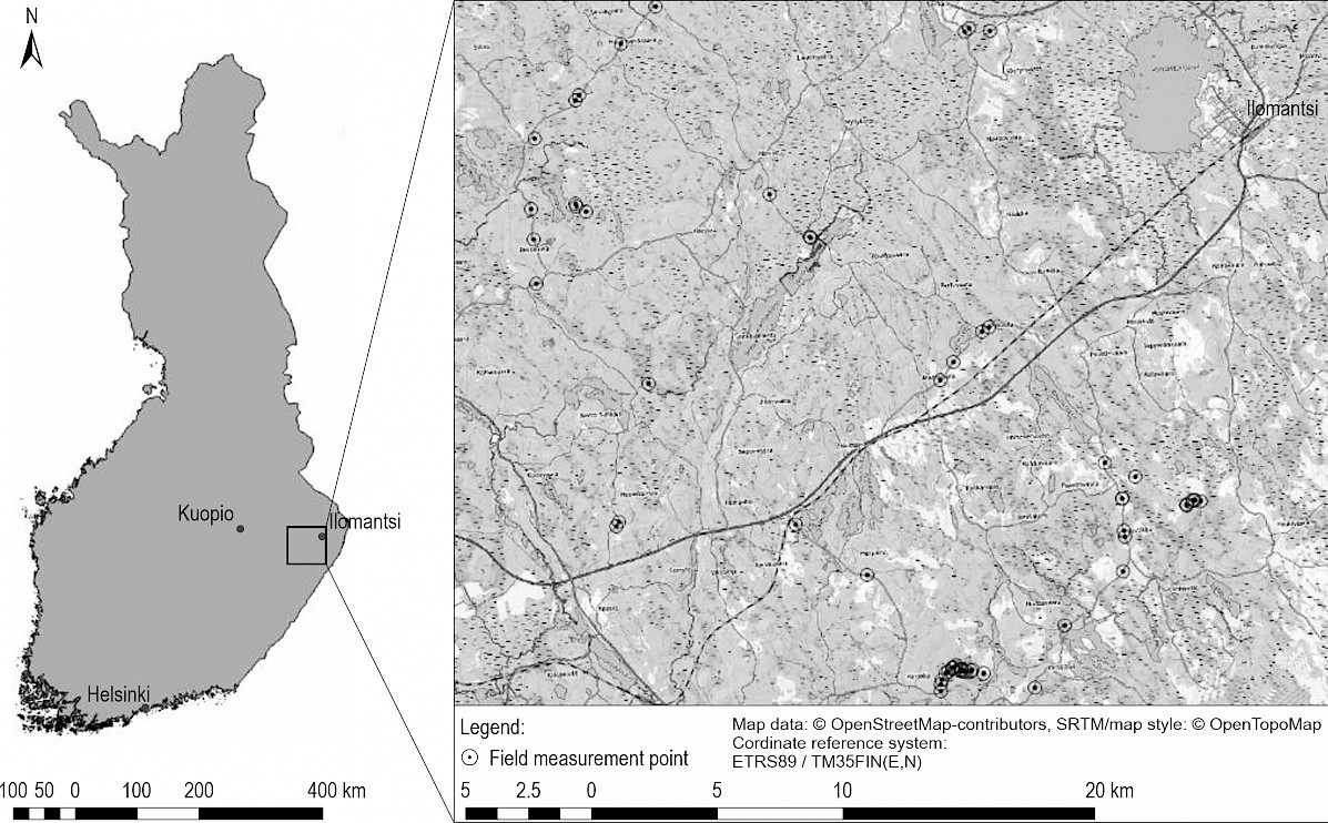
Fig. 1 Location of study area (left) and a detailed view of study area and location of sampling points (right). Field data sampling points are marked with a circle

Spatial data from the study area was available in the form of 3D location data from Airborne Laser Scanning (ALS). Despite the superior quality of UAV data, we decided to use public available ALS data, because the latter covers bigger areas and is more cost effective when analysing bigger forest road networks. The ALS campaign was carried out by Terratec AS between May 2022 and the beginning of June 2022 as part of the national land survey campaign of Finland. Data was collected with a RIEGL VQ–1560 II–S Laser Sanner, mounted on a Cessna 208B airplane. Scanning angle was 20 degree with a flight altitude of 2100 meters from average ground level at a speed of 155 km/h. The scanner operated with a pulse frequency of 1.62 MhZ capturing data with 20% overlap. The ALS point data was collected with an average position errors of 5 cm vertically and 4 cm horizontally. The average point density was about 5 points m per square meter. With the help of the Terrscan software plugin in Microstation, the Laser scan data was further processed into a Digital Terrain model with 10 cm resolution using the lowest return points (z–min). The raster data type was chosen over ground laser scan points due to simpler data handling and necessary point interpolation. The DEM was created using triangulation of the classified ground returns. Field data were collected for three days between September and October 2022. Damaged road locations were identified by driving across the study area with visual inspection of road condition. Road damage was defined as local depression of the road surface where driving speed with a common automobile had to be reduced significantly in order to avoid damage to the vehicle. In total, 69 locations were semi-randomly selected by stratification according to the attribute range found in the field. Road depression depths were measured on 40 forest roads. The use of field maps ensured that the data were evenly distributed over the target area in order to capture a wide variety of road structures and conditions. For later evaluation, the damage type was determined and a photo was taken at each damaged road location.

To determine the depth of the depressions in the road, a 1.3 m straight wooden pole was placed horizontally on the damaged area. Next, the maximum distance from the bottom of the depression to the lower edge of the pole was measured with a tape measure and rounded up to whole centimetres, as indicated in Figure 3. The location of the deepest depression was then captured with a Trimble Geo7X Handheld GNSS System attached to a Trimble Zephyr Antenna mounted on a 4 m monopod equipped with a level. Captured points were further corrected using the Differential Correction technique with Trimble GPS Pathfinder Office v. 5.60.

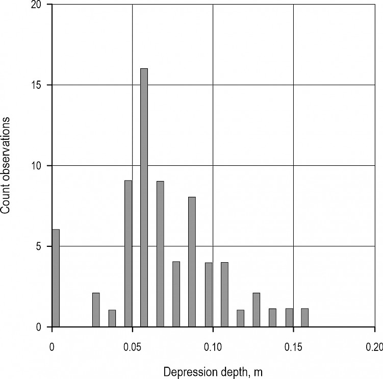
Fig. 2 Distribution of road damage depth measurements, m

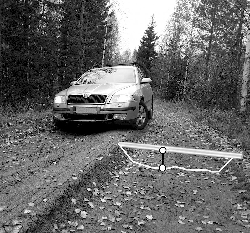
Fig. 3 Schematic view of the applied collection method. White bar represents a straight pole, white line the road surface profile. Maximum distance between road profile and pole is indicated by black line

In total, 63 damaged points were captured. Additional 6 plots were established on reference roads with no damage. Location position error of the GNSS coordiantes ranges from 0.1 to 0.8 m. Measured depressions ranged from 3 cm to 16 cm and most depressions were between 5 and 10 cm deep.

Four interpolation methods based on a DTM in raster format were selected to estimate the optimal road surface without damage, as indicated in Fig. 4.

The methods were as follows:

Maximum elevation value inside a predefined moving raster window

Mean elevation value of a predefined moving raster window

Triangulation (Peucker et al. 1979) of maximum DEM values

Spline interpolation (Haber et al. 2008) of maximum DEM values

Four versions with different window sizes were prepared from each interpolation candidate to determine the best fit for damage detection. The variables are shown in Table 1. For each element in the variable list, one interpolated raster with 10 cm ground sampling distance was created and subtracted from the original DTM. All interpolation tools were performed in Quantum-GIS version 3.12 and version 3.28.

Table 1 Determined input variables based on interpolation (grey) and ALS point information (white)

Variable source	Window size, pixel	Tool	Resulvation, meter	Variable name
Maximum filter	5,10,15,20	Whitebox–tools	0.1	Max5, Max10, Max15, Max20
Mean filter	5,10,15,20	Whitebox–tools	0.1	Avg5, Avg10, Avg15, Avg20
Triangulation	5,10,15,20	SAGA–GIS	0.1	Tri5, Tri10, Tri15, Tri20
Cubic spline	5,10,15,20	SAGA–GIS	0.1	Spl5, Spl10, Spl15, Spl20
Point density, m²	X	Terrascan	1	PD
Intensity	X	Terrascan	0.1	Int

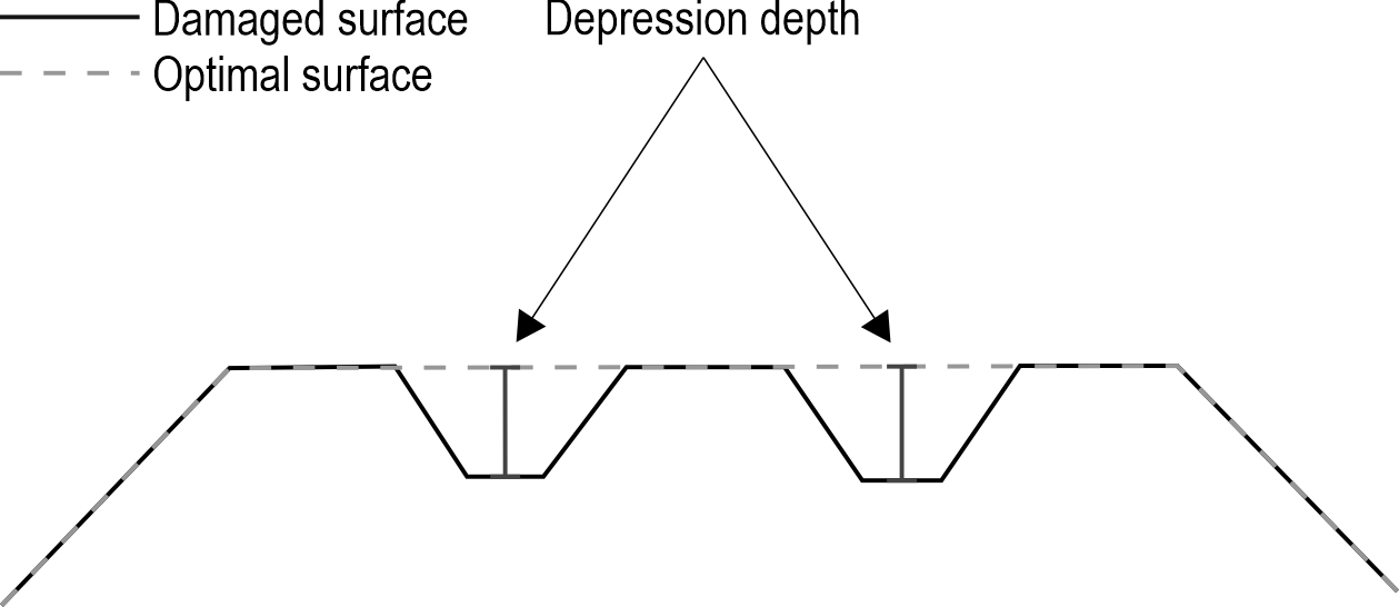
Fig. 4 Schematic overview of underlying methodology

The interpolated data, maximum laser return intensity and ground point density m2 were joined to the sample plots using QGIS zonal statistics. The measured sample points were buffered by the individual maximum x, y positioning error and a 20 cm buffer to account for coordinate reference system uncertainties. Furthermore, the greatest difference between the DEM and the interpolated raster image was attributed to the created polygons. In sum, 18 predictors were defined as displayed in Table 1, and used to create a linear mixed effect model (LMM).

LMM is a technique that uses independent variables, also called fixed factors to predict the outcome of a single dependend variable by fitting a linear model to data points. Opposed to simple linear regression, this method uses a second variable also called random factor to account for group-wise effects, in our example location expressed as road id. The equation with the best performing variables is shown below.

 (1)

Where:

DD depression depth, m

Avg15 interpolation difference to DTM using a mean filter and a 15 pixel (1.5 m) sized window, m

Spl15 interpolation difference to DTM using spline and a 15 pixel sized window, m

PD point density per square meter

Roadid random factor

b0-3 coefficients.

Before the model was created, intensely vegetated roads were removed from the analysis because of ground classification issues. Additionally independent variables with high correlation (Pearson >0.8) have been excluded. Using the two directional exhaustive search methods in the regsubset function (R package leaps) for variable selection, the best performing candidates were selected based on the minimised sum of squares. The determined variables were then tested for accuracy using K-Fold cross validation, splitting the dataset in 10 groups whereas 10% of the data was used for testing. The selection of the final model was based on the smallest Root Mean square error (RSME) and significance p<0.05.

The equation for determining this measure is defined as:

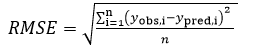  (2)

Where:

yobs,i - observed value, m

ypred,i - predicted value, m

n - total number of observations.

Using a linear mixed model (LMM), we investigated whether single roads had a random influence on the estimation process, by allowing a variable slope coefficient amongst the observations per group. Using the lmer function of the package lme4, as well as the lme function (nlme) in R, a model was constructed using the variables that were determined in the previous steps with road id as random variable. For each model, different statistical measures have been calculated to compare the performance for each version, as well as the performance with and without the random effect in question. Testing all the models with the help of the likelihood ratio test using the anova function in R against a Null model indicated that all results are significantly different from chance (p<0.05). R2 values have been calculated using the r.squaredGLMM function of the MuMIn package in R. R2 is calculated in two categories, R2 marginal (R2GLMM(m)) and R2 conditional (R2GLMM(c)).

The R2 marginal is a measure that represents the variance explained by the fixed effects, whereas R2 conditional incoorporates both random and fixed effects combined. Both measures are in the package documentation defined as:

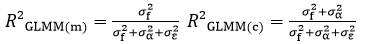 (3)

Where:

σf2 variance of fixed effect

σα2 variance of random effect

σϵ2 variance of our observations.

To eliminate temporal discrepancy and to assess accuracy, the depth of the detected depression was manually measured in the DEM by drawing a profile over each sample point (Digital Twin reference) using the QGIS Plugin »Profile tool«. Then, a virtual 1.3 m line was laid over the depression and the maximum distance to the bottom of the depression was measured. With the help of a linear mixed effect model, it was tried to explain the depression depth in the field, with the values virtually measured in the DTM (deviation values are shown in Fig. 4). Then, sample plots in the range 0.13 m to 0.05 m of the differences were inspected by evaluating the pictures taken from the specific segments of the road to determine the likelihood that the damage or its intensification occurred after collection during the ALS campaign. If damage or its intensification was deemed likely after collection, these points were removed from the multiple regression analysis. In total, 10 of the 13 plots were identified to have a high probability that the damage or its intensification occurred after data collection. Overall, including two erroneous points (missing data, undetectable crack), the cleaned dataset was reduced from 69 to 48 sample points.

3. Results

A comparison of the measured digital and manual values is shown in Table 2. Almost all (apart from good roads) of the depth values in the digital twin were less than those measured in the field. Qualitative differences between the groups can be recognised when the values are grouped by damage type. Measurements of the wheel grooves appeared slightly less dispersed than those of potholes or water channels (Fig. 5 and Table 2). This might be attributed to the different surface sizes (depth + area) of damage type.

Plotting the field data against the digital measured values showed that a maximum R2 of 0.66 with a residual standard error of 2 cm could be reached. This indicates the limit of the maximum reachable accuracy.

 

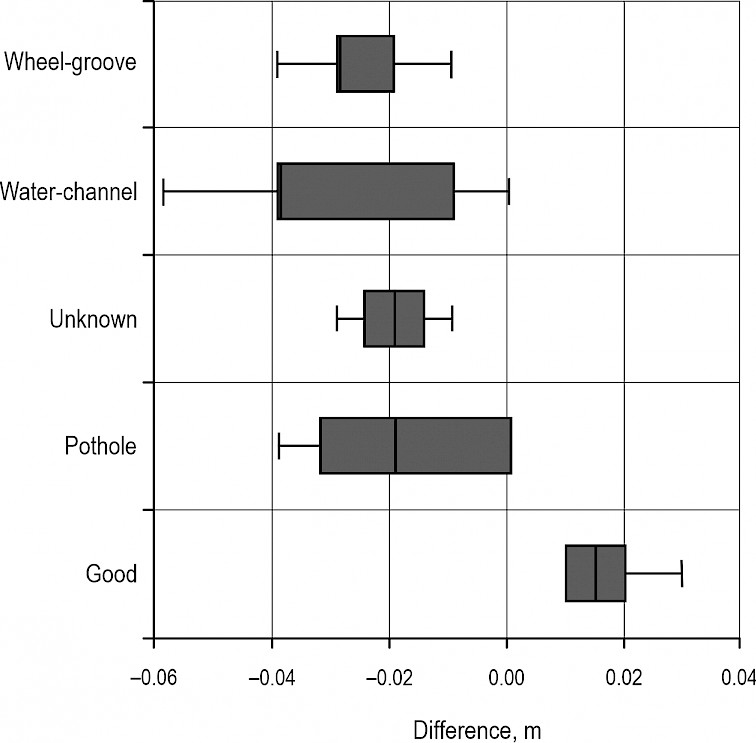
Fig. 5 Boxplots displaying differences between virtual and field measured plots, grouped by damage type. Data from Table 2

Table 2 Comparison of differences between virtual and field measured plots in meter, grouped by damage type

Damage type	Good	Wheel groove	Unknown	Pothole	Water channel
Count	6	15	2	16	9
Mean	0.017	–0.027	–0.02	–0.019	–0.029
Std. Dev.¹	0.008	0.011	0.014	0.017	0.02
MAD²	0.005	0.01	0.01	0.02	0.02
Minimum	0.01	–0.04	–0.03	–0.04	–0.06
Maximum	0.03	0	–0.01	0	0
1 Standard deviation 2 Median absolute deviation

The removal of vegetated roads from the sample points increased the proportion of variation in the response variable (depression depth) explained by the fixed factors (See Table 3). Compared to the model construction without filtering, the marginal R2, which represents the variance explained by the fixed effect, increased from 0.14 to 0.32, while the influence of location (road id) decreased from 62% to 29%. Combining the fixed effects with the random effect (variable slope over road id), the conditional R2, representing the variance explained by the entire model, improved from 0.36 to 0.45 without an effect on the error term RSME.

A closer look into Table 3 also indicates that the removal of sample points, where it was highly likely that a road damage happened after ALS data collection, could increase the accuracy even further. In our study, point density per square meter (PD), the 150 cm window size mean and spline interpolation product (Mean15, Spl15) were identified to provide the most accurate results from all observed variable candidates. Compared to the sample points without vegetation, the marginal R2 improved from 0.32 to 0.44. Location could increase the conditional R2 from 0.45 to 0.58, indicating that about one fourth (24%) of variability of variance could be explained by local factors.

A visual analysis of the final model indicates that the model residuals are approximately normally distributed, Fig. 6 (left side). Plotting the model residuals vs the fitted values shows that the first six points on the X-axis falling below the zero line deviate from the rest of the points. This indicates that at least for smaller depression depths a threshold linear model or a nonlinear model might be more adequate to describe depression depth. Because of the small sample size of 48 and no actual measurements from 1 to 4 cm, the results for smaller depression depths up to 4 cm have to be interpreted with care. Compared to previous versions, the final model using three variables and location as random effect appears to decrease the Root Mean Square error to 1.8 cm.

Constructing a reference model using the field and digitally measured depths gave further insights into the limits and reliability of the applied method. Location/Road id explains up to a quarter of variability in the data (~30%), corresponding with previous models, where data filtering was applied (24–29%). Compared to the best performing model (R2 0.44), our reference model indicates a higher Marginal R2 of 0.61. Incorporating a variable slope over road id, using the mixed effect model approach, leads to a maximum conditional R2 of 0.87, an improvement about 30% from 0.58. Comparing the root mean square error with our created models, it is noticeable that the error term with 2.7 cm increased about 1 cm compared to our best model.

Table 3 Model results using different data filtering methods. RMSE (cm) denotes the residual mean standard error for the model with fixed effect (Cond=Conditional) and without (Marg=Marginal). Random% and Fixed% displays the share of variability explained by random and fixed factors

Method	Predictor	RMSE–Cond	R2–Cond	R2–Marg	RSME–Marg	Random, %	Fixed, %	N
No filter applied	Spl15	2.2	0.36	0.14	3.0	62	38	67
No vegetation	Pd, Tin15	2.2	0.45	0.32	2.6	29	71	58
No veg./Pict. sel.*	Pd, Mean15, Spl15	1.8	0.58	0.44	2.4	24	76	48
Optimal max.	Virtual	2.7	0.87	0.61	1.9	30	70	48
*No vegetation/Pictures indicating road damage after ALS data collection removed

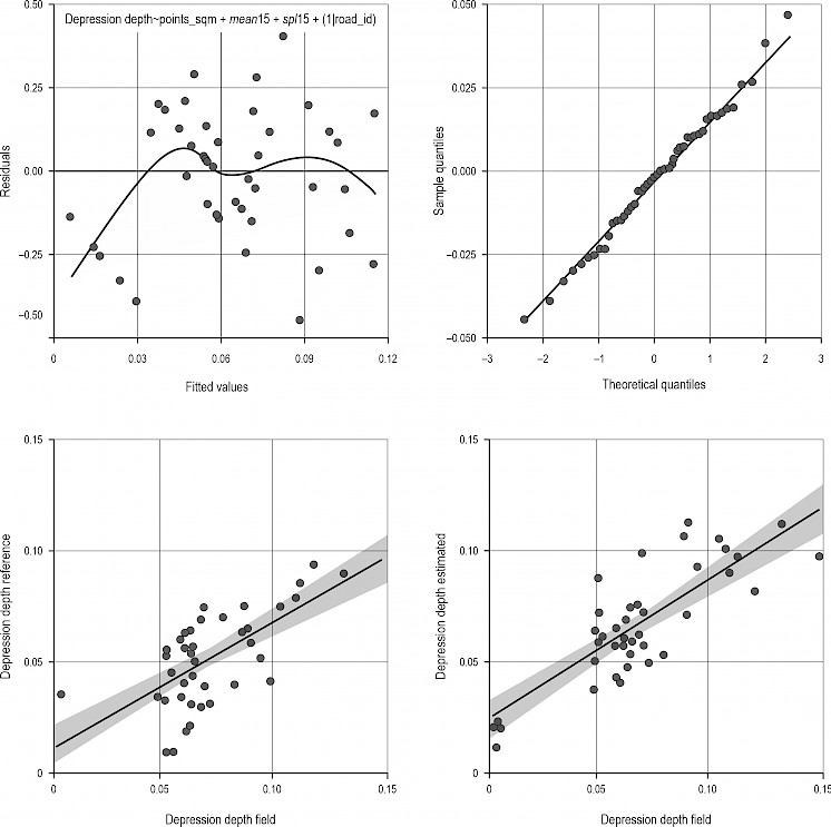
Fig. 6 (Upper left) Model summary displaying the best performing model residuals plotted against fitted values. Grey line represents the weight of the fit. (Right left) Q-Q plot for comparing model residual quantiles to quantiles of a normal distribution. (Bottom left) Depth measurements from the field plotted against digital reference values. Black line indicates the linear trend of the data, accompanied by a standard error term in grey. (Bottom right) Depth measurements from the field plotted against depth measurements estimated by best performing model. Black line indicates the linear trend of the data, accompanied by a standard error term in grey

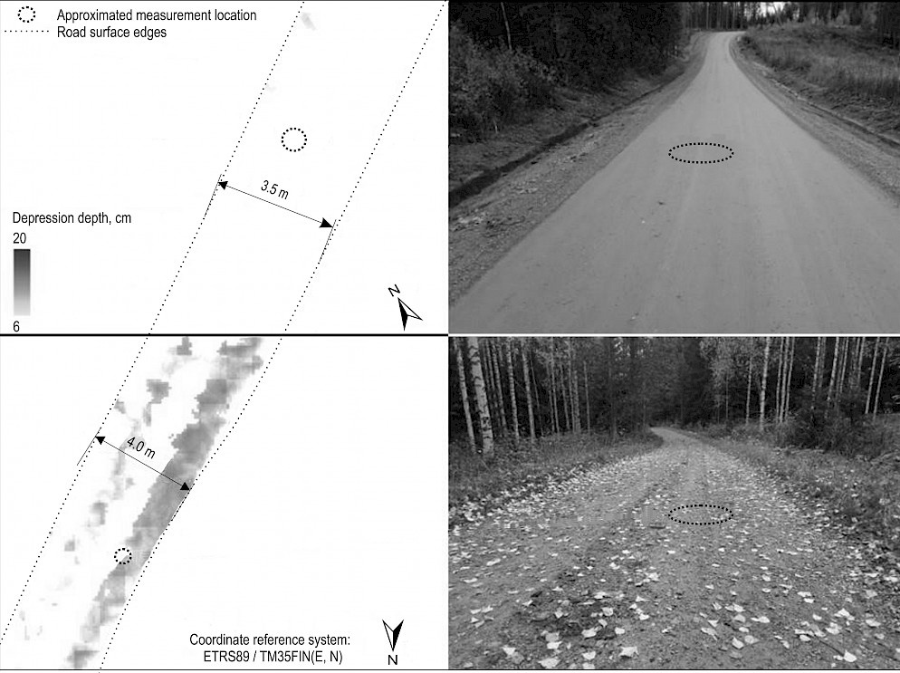
Fig. 7 Estimated road damage (depression depths) for a road in good condition (upper) and bad condition (lower), with the corresponding photo from the road taken during field data collection

4. Discussion

In Finland, the operational wood transportation network was mostly constructed between 1960 and 1990 and the planned structural life of the roads was expected to be 20–30 years. As such, many of these roads are now reaching the end of their life cycle (Kaakkurivaara and Uusitalo 2011). Several methods have been tested to estimate forest road quality, such as ranking from direct measurements to estimation of the factors that influence road quality, such as wetness or soil type.

Waga et al. (2020), for example, showed that forest road condition could be linked to soil wetness, while Vuorimies et al. (2015) linked road condition to traffic load. Still, there is a lack of studies related to a direct quality estimation of forest road condition. Moreover, there is an urgent need for a cost-efficient monitoring system to maintain the trafficability of road networks at a reasonable level, although this problem might be overcome with the arrival of three-dimensional laser scanning data in recent decades in combination with increased accuracies and higher pulse densities.

To utilize this development, we explored the relationship between LiDAR responses and road depressions. We assumed that the difference in the damaged road surface from its optimal shape could lead to insights into where the damage occurred and its intensity (depth).

By creating a digital twin of the field measurements, it was possible to estimate how well the data would be able to predict the intensity of road depressions. In the most optimal case, a linear mixed effect model could achieve an R2 of 0.87 with and 0.66 without the random factor having a residual mean standard error (RSME) of 1.9 to 2.7 cm on unvegetated forest roads. The best performing model determined in our study using ALS derived variables reached an R2 of 0.58 and 0.44 with an RSME of 1.8 to 2.4 cm.

Road location appears to have a significant influence on the prediction of depression depths. Comapring the models with and without the random variable led to up to 30% more informational value when incorporating road location into the analysis. However, it has to be noted that many roads had only single observations, thus the location depended variability should be interpreted with care.

Our study has also shown the practical application and limits of medium density ALS data for the detection of road damage depth on forest roads. The greatest source of uncertainty appeared to be the data itself. Not only does the relatively small dataset introduce some uncertainty, but the 6 month temporal discrepancy between the ALS campaign and the field data collection must also be taken into account. Damage or intensification could happen within the described time period, and not be recognised in the field. Also, it was observed that extensive vegetation on, or near the road surface, had a substantial impact on the estimation of damage depth, due to misclassification of these areas as ground. This observation corresponds to the findings of another study (Hrůza et. al. 2018), where vegetation had a substatial impact on ALS derived road profiles.

Removal of sample plots affected in this way led to an improvement in the R2 value and the residual standard error in our model. However, the author of a previous study reported an RSME of 0.14 m comparing ALS derived road cross sections to the ground reference, which is not evident in our study, reaching error terms between 0.02 to 0.03 m.

Therefore, there is a need to control the estimation process to detect the factors that negatively influence the estimates. A detection method for vegetated roads and a separate model for those cases could be developed to overcome this limitation.

Taking the vertical positioning error and point density into account, road damage with a greater surface area (depth + area), such as wheel grooves, might be more accurately detected than damage with a smaller surface area. The reliability of estimation and the overall underestimation of the depression depth using the reference data would indicate that a point density of 5 points m2, on average, is insufficient to capture the full extent of each damage. Although basic road features could be extracted from low point densities (White et al. 2010), many studies use high density laser scanning data to analyse road surface structures (Yadav et al. 2018, Husain et al. 2018, Feng et al. 2021). The finding that higher point densities are required to assess surface damage has also been reported in other studies (e.g. Waga 2021), where the best results were achieved using high-density datasets.

To overcome this problem, it might be appropriate to change the scope of the study from a single damage description to an evaluation of the whole road surface structure. For example, the deviation of measured values to an interpolated road surface could be summarised in a segment-wise manner and related to a location depended variable such as road geometry parameters, soiltype or surface material. Road width could be incoorporated as well, since it can be derived from ALS data of similar quality (Karjalainen et. al 2024) and could give information about road condition (Workman et al. 2023). In this way, there would be no need for the collection of higher density point data. Furthermore, the results could be used to build a framework for road damage detection and damage assessment, without the need for manual measurements.

Another approach could be the determination of surface damage using surface roughness, as indicated in multiple research projects (e.g. Marinello et al. 2017, Aleadelat et al. 2018, Alhasan et al. 2015). By using roughness information from ALS data and training the results with ground-collected vibration data, the direct prediction of road damages could be improved.

Methods using machine learning might also be tested in combination with previous approaches, to detect road damages. A study sing UAV aquired imagery has proven suffiecient results in detecting harvester ruts in Norwegian forests with a detection rate of almost 80% (Bhatnagar et al. 2022). Given the similiarity of damage compared with those of forest roads, it might also be worth to combine multiple datasets and test for detectability of damages using modern classification methods.

Thus, while remote sensed data might not be as accurate as ground-based methods, it could fill the gap in areas where vehicle access is difficult or where the application of ground-based methods is not economically feasible.

Acknowledgements

The research was funded by the University of Eastern Finland and Oy Arbonaut Ltd,, and is part of a graduate thesis of the main author.

5. References

Aleadelat, W., Wright, C.H.G., Ksaibati, K., 2018: Estimation of Gravel Roads Ride Quality Through an Android-Based Smartphone. TRR 2672(40): 14–21. https://doi.org/10.1177/0361198118758693

Alhasan, A., White, D.J., De Brabanter, K., 2015: Quantifying Roughness of Unpaved Roads by Terrestrial Laser Scanning. TRR 2523(1): 105–114. https://doi.org/10.3141/2523-12

Bhatnagar, S., Puliti, S., Talbot, B., Heppelmann, J.B., Breidenbach, J., Astrup, R., 2022: Mapping wheel-ruts from timber harvesting operations using deep learning techniques in drone imagery. Forestry 95(5): 698–710. https://doi.org/10.1093/forestry/cpac023

Dong, D., Li, Z., 2021: Smartphone Sensing of Road Surface Condition and Defect Detection. Sensors 21(16): 5433. https://doi.org/10.3390/s21165433

Edvardsson, K., Lundberg, T., Sjögren, L., 2015: Objective measurement method for assessment of gravel road condition. Statens väg-och transportforskningsinstitut.

Feng, Z., El Issaoui, A., Lehtomäki, M., Ingman, M., Kaartinen, H., Kukko, A., Savela, J., Hyyppä, H., Hyyppä, J., 2022: Pavement distress detection using terrestrial laser scanning point clouds–Accuracy evaluation and algorithm comparison. ISPRS J. Photogramm. 3: 100010. https://doi.org/10.1016/j.ophoto.2021.100010

Haber, J., Zeilfelder, F., Davydov, O., Seidel, H.P., 2008: Smooth approximation and rendering of large scattered data sets. From Nano to Space. Springer 127–143. https://doi.org/10.1007/978-3-540-74238-8_11

Heidari, M.J., Najafi, A., Borges, J.G., 2022: Forest roads damage detection based on deep learning algorithms. Scand. J. For. Res. 37(5–8): 366–375. https://doi.org/10.1080/02827581.2022.2147213

Hoffmann, S., Schönauer, M., Heppelmann, J., Asikainen, A., Cacot, E., Eberhard, B., Hasenauer, H., Ivanovs, J., Jaeger, D., Lazdins, A., Mohtashami, S., Moskalik, T., Nordfjell, T., Stereńczak, K., Talbot, B., Uusitalo, J., Vuillermoz, M., Astrup, R., 2022: Trafficability Prediction Using Depth-to-Water Maps: The Status of Application in Northern and Central European Forestry. Curr. For. Rep. 8(1): 55–71. https://doi.org/10.1007/s40725-021-00153-8

Hoseini, M., Puliti, S., Hoffmann, S., Astrup, R., 2024: Pothole detection in the woods: A deep learning approach for forest road surface monitoring with dashcams. Int. J. of Forest Eng. 35(2): 303–312. https://doi.org/10.1080/14942119.2023.2290795

Hrůza, P., Mikita, T., Tyagur, N., Krejza, Z., Cibulka, M., Procházková, A., Patočka, Z., 2018: Detecting Forest Road Wearing Course Damage Using Different Methods of Remote Sensing. Remote Sens. 10(4): 492. https://doi.org/10.3390/rs10040492

Husain, A., Vaishya, R.C., 2018: Road surface and its center line and boundary lines detection using terrestrial Lidar data. Egypt. J. of Remote Sens. 21(3): 363–374. https://doi.org/10.1016/j.ejrs.2017.12.005

Karjalainen, T., Karjalainen, V., Waga, K., Tokola, T., 2024: Predicting the roadway width of forest roads by means of airborne laser scanning. Int. J. Appl. Earth Obs. 133: 104109. https://doi.org/10.1016/j.jag.2024.104109

Kelesakis, D., Marthoglou, K., Tokmaktsi, E., Tsiros, E., Karteris, A., Stergiadou, A., Kolkos, G., Daras, P., Grammalidis, N., 2024: Forest/rural road network detection and condition monitoring based on satellite imagery and deep semantic segmentation. ISPRS Photogramm. Remote Sens. 10: 81–88. https://doi.org/10.5194/isprs-annals-X-4-W4-2024-81-2024

Kiss, K., Malinen, J., Tokola, T., 2016: Comparison of high and low density airborne lidar data for forest road quality assessment. ISPRS Photogramm. Remote Sens. 3: 167–172. https://doi.org/10.5194/isprsannals-III-8-167-2016

Marinello, F., Proto, A.R., Zimbalatti, G., Pezzuolo, A., Cavalli, R., Grigolato, S., 2017: Determination of forest road surface roughness by Kinect depth imaging. Ann. For. Res. 60(2): 217–226. https://doi.org/10.15287/afr.2017.893

Salmivaara, A., Launiainen, S., Perttunen, J., Nevalainen, P., Pohjankukka, J., Ala-Ilomäki, J., Sirén, M., Laurén, A., Tuominen, S., Uusitalo, J., Pahikkala, T., Heikkonen, J., Finér, L., 2020: Towards dynamic forest trafficability prediction using open spatial data, hydrological modelling and sensor technology. J. Forest Res. 93(5): 662–674. https://doi.org/10.1093/forestry/cpaa010

Skorseth, K., 2000: Gravel roads: maintenance and design manual. US Department of Transportation, Federal Highway Administration. https://www.epa.gov/nps/gravel-roads-maintenance-and-design-manual

Vuorimies, N., Kolisoja, P., Kaakkurivaara, T., Uusitalo, J., 2015: Estimation of the Risk of Rutting on Forest Roads during the Spring Thaw. TRR 2474(1): 143–148. https://doi.org/10.3141/2474-17

Waga, K., Malinen, J., Tokola, T., 2020: A Topographic Wetness Index for Forest Road Quality Assessment: An Application in the Lakeland Region of Finland. Forests 11(11): 1165. https://doi.org/10.3390/f11111165

Waga, K., Malinen, J., Tokola, T., 2021: Locally invariant analysis of forest road quality using two different pulse density airborne laser scanning datasets. Silva Fenn. 55(1): 10371. https://doi.org/10.14214/sf.10371

White, R.A., Dietterick, B.C., Mastin, T., Strohman, R., 2010: Forest Roads Mapped Using LiDAR in Steep Forested Terrain. Remote Sens. 2(4): 1120–1141. https://doi.org/10.3390/rs2041120

Workman, R., Wong, P., Wright, A., Wang, Z., 2023: Prediction of Unpaved Road Conditions Using High-Resolution Optical Satellite Imagery and Machine Learning. Remote Sens. 15(16): 3985. https://doi.org/10.3390/rs15163985

Yadav, M., Lohani, B., Singh, A.K., 2018: Road surface detection from mobile lidar data. ISPRS Photogramm. Remote Sens. 4: 95–101. https://doi.org/10.5194/isprs-annals-IV-5-95-2018

© 2025 by the authors. Submitted for possible open access publication under the
terms and conditions of the Creative Commons Attribution (CC BY) license (http://creativecommons.org/licenses/by/4.0/).

Authors' addresses:

Maik Grabow, MSc *

e-mail: maik.grabow@uef.fi

Prof. Timo Tokola, PhD

e-mail: timo.tokola@uef.fi

University of Eastern Finland

Faculty of Sciences

Forestry and Technology

Yliopistokatu 7

FIN-80100 Joensuu

FINLAND

Vesa Leppänen

e-mail: vesa.leppanen@arbonaut.com

Arbonaut Ltd

Kaislakatu 2

FIN-80130 Joensuu

FINLAND

* Corresponding author

Received: September 28, 2023

Accepted: January 08, 2025

Original scientific paper

7

Download PDF