On the Importance of Integrating Transportation Costs into the Tactical Forest Harvest Scheduling Model

In tactical forest management planning, the decisions required to meet the strategic plan are made, and these include: i) scheduling of spatially explicit harvest-blocks; ii) construction of a road-network required to access these blocks; and iii) transportation costs within the tactical forest planning area (hereafter only referred to as transportation costs) that emerge from the first two decisions. These three decisions are interdependent and should therefore be integrated in any optimization model. At present, this integration is not fully made. This is because: i) the integrated model is NP-hard, and exact solutions are not feasible for large and medium-sized forests; and ii) metaheuristic search algorithms, which can be used on larger forests, have not integrated transportation costs realistically.

The economic consequences of not integrating transportation costs into tactical planning models has not been quantified and evaluated by researchers; and the objective of this paper is to fill this gap in knowledge. To this end, an exact solution approach is used to solve and compare two integrated models: i) a model in which transportation costs are included in the objective function, and b) a model in which transportation costs are excluded from the objective function. The models were applied to three forests ranging in area from 6628 to 19,677 ha.

Results show that: i) the model which included transportation costs yielded solutions with major reductions in both transportation and total costs; and ii) that, as the forests to which the model was applied tripled in area (from 6628 ha to 19,677 ha), the percent reduction in total costs increased disproportionately – more than fivefold (from 3.9% to 21%). These results are important, for they indicate that the integration of transportation costs into a tactical planning model is of major economic consequence.

On the Importance of Integrating Transportation Costs into Tactical Forest Harvest Scheduling Model

Nader Naderializadeh, Kevin A. Crowe, Reino Pulkki

Abstract

In tactical forest management planning, the decisions required to meet the strategic plan are made, and these include: i) scheduling of spatially explicit harvest-blocks; ii) construction of a road-network required to access these blocks; and iii) transportation costs within the tactical forest planning area (hereafter only referred to as transportation costs) that emerge from the first two decisions. These three decisions are interdependent and should therefore be integrated in any optimization model. At present, this integration is not fully made. This is because: i) the integrated model is NP-hard, and exact solutions are not feasible for large and medium-sized forests; and ii) metaheuristic search algorithms, which can be used on larger forests, have not integrated transportation costs realistically.

The economic consequences of not integrating transportation costs into tactical planning models has not been quantified and evaluated by researchers; and the objective of this paper is to fill this gap in knowledge. To this end, an exact solution approach is used to solve and compare two integrated models: i) a model in which transportation costs are included in the objective function, and b) a model in which transportation costs are excluded from the objective function. The models were applied to three forests ranging in area from 6628 to 19,677 ha.

Results show that: i) the model which included transportation costs yielded solutions with major reductions in both transportation and total costs; and ii) that, as the forests to which the model was applied tripled in area (from 6628 ha to 19,677 ha), the percent reduction in total costs increased disproportionately – more than fivefold (from 3.9% to 21%). These results are important, for they indicate that the integration of transportation costs into a tactical planning model is of major economic consequence.

Keywords: harvest-scheduling model, tactical planning, transportation costs, integer programming, fixed charge network design model

1. Introduction

In tactical forest management planning, among others, the following decisions are made to implement the forest strategic plan: i) scheduling of spatially explicit harvest-blocks (based on discounted revenue per block); ii) construction of a road-network required to access these scheduled blocks (based on discounted cost per km of constructed road); and iii) transportation of the scheduled harvest of wood through the constructed road network (based on cost per m3 per km). Hence, the two major costs resulting from tactical-level planning arise from constructing forest roads and transporting harvested wood through the road-network within the tactical forest planning area (hereafter only referred to as transportation costs) (Bjørndal et al. 2012). The economic importance of the integrated tactical planning problem has, therefore, warranted extensive research on optimization models of this planning problem (Bettinger and Chung 2004).

The first major advance in modeling the tactical planning problem in forestry was based on the insight that, since the optimal locations of both cut-blocks and roads are interdependent (given an objective to maximize revenue minus cost), a model that solves both of these allocation problems simultaneously performs better than a model that first allocates the scheduled cut-blocks, and then designs an optimal road network: i.e., a sequential approach (e.g., Weintraub and Navon 1976, Kirby et al. 1980, 1986, Jones et al. 1986). For example, Jones et al. (1986) showed that solutions resulting from a model in which decisions when harvesting, road construction and transportation were integrated, resulted in 15% to 45% lower costs than the solutions generated when these decisions were made sequentially.

A second major advance of tactical planning models occurred in the early 1990s, when models were adapted in response to the introduction of new environmental objectives that required spatial constraints on harvesting (Bettinger and Chung 2004). For example, tactical models were developed to include adjacency constraints (i.e., constraints ensuring that no set of adjacent cut-blocks be harvested in the same period in order that opening sizes not exceed a defined limit in area). This problem has been addressed extensively by researchers (e.g., Goycoolea et al. 2009). The introduction of spatial planning constraints required the introduction of binary decision variables to represent the scheduling of harvest-blocks, and thereby transformed the tactical harvest-scheduling model into a NP hard model (Murray 1999); i.e., the model required exponentially more computing time to be solved as the size of the problem instance increased.

A third major advance in the tactical planning model occurred when metaheuristic algorithms were developed to solve the model. Given the computational challenge of solving the spatially explicit harvest-scheduling problem, there was an expansion of research in the 1990s, and beyond, into the design and application of metaheuristic search algorithms for solving this problem. This research was justified because exact solution methods, although capable of finding mathematically optimal solutions to the spatially constrained tactical model, can only solve problem instances that are quite small relative to the size of problems encountered by practicing planners. Hence, the primary advantage of using metaheuristic solution methods is that, although their solutions were not demonstrably optimal, realistically-sized problem instances could be solved by them.

The solutions of models of the integrated harvest-scheduling and road network design problem using metaheuristic algorithms differed slightly from models using exact solution methods. On the one hand, the models solved using exact methods had three key elements in their objective function: to maximize (i) the revenue from harvests, minus (ii) the cost of constructing roads and (iii) the cost of transporting harvested wood. The representation of transportation costs in these models was based on the flow of harvested wood through the constructed road network: i.e, the flow from supply nodes, through the road-network, to demand nodes, using standard network-flow constraints (e.g., Guignard et al. 1998, Andalaft et al. 2003, Silva et al. 2010, Veliz et al. 2015, Naderializadeh and Crowe 2018). On the other hand, models solved using metaheuristic algorithms either: (a) did not represent transportation costs in the objective function (e.g., Nelson and Brodie 1990, Murray and Church 1995, Clark et al. 2000, Richards and Gunn 2000, 2003), or (b) if transportation costs were represented by network flow variables, road-construction decisions would not be integrated with transportation decisions (e.g., Bettinger et al. 1998, Chung et al. 2012).

The reason metaheuristic algorithms have not, thus far, been used to solve models where construction, harvesting and transportation decisions are fully integrated, is the computational burden: i.e., computing time required to solve such models. The computational challenge exists for metaheuristics because such an integration would require nesting a fixed charge network design model (see Magnanti and Wong 1984) within a spatially explicit harvest scheduling model; and both of these models are NP-hard (Martel et al. 1998, Magnanti and Wong 1984). Hence, for each candidate harvest-schedule, evaluated by a metaheuristic algorithm, a fixed charge network design model (see Magnanti and Wong 1984) must be solved. Since several million candidate harvest-schedules are typically evaluated for a standard problem instance when using a metaheuristic algorithm, the computational burden of solving an NP-hard problem nested within another NP-hard slows the metaheuristic search to an ineffective exploration of search space over time.

There has been no quantitative research addressing the economic importance of including versus excluding transportation costs in the integrated tactical forest planning model. This inquiry is important because: (a) transportation costs entailed by a tactical plan are of major economic significance, and (b) metaheuristic algorithms do not realistically integrate transportation costs.

The economic consequences of not integrating transportation costs into tactical planning models has not been quantified and evaluated by researchers. Thus, the objective of this paper is to fill this gap in knowledge. An exact solution approach is used to solve and compare two integrated models: i) a model in which transportation costs are included in the objective function, and b) a model in which transportation costs are excluded from the objective function. The models are applied to three forests areas 6628, 12,622 and 19,677 ha in size, and their solutions were analyzed, mapped and compared based on income minus road construction and transporting costs.

2. Methods

The mathematical formulation of the integrated model, used in this paper, is the same formulation presented by Naderializadeh and Crowe (2018b). This formulation of the tactical planning model differs from prior published formulations in the following important respects.

First, the candidate roads in this model do not represent individual arcs, but rather, represent a set of operational-scale arcs that are constrained to meet the horizontal and vertical design-standards of forest roads (see Anderson and Nelson 2004). Hence, in this model, when a polygon is scheduled for harvest, and the construction of a road is thereby triggered, the full set of operational-scale arcs, comprising that road, is also triggered for construction. This approach was taken for two reasons: i) it can be useful if a tactical plan, handed down to the operational scale, contains roads that are designed to meet operational road design standards; and ii) the formulation facilitates using a dense set of candidate roads in the problem instance; and a dense set of candidate roads facilitates more alternatives by which a road network can be designed to minimize construction and transportation costs (Naderializadeh and Crowe 2018b).

Second, the decision variable used to represent the construction of a candidate road is a directed arc, instead of an undirected edge. Third, strengthening constraints are used that exploit the directed attribute of the candidate roads. Fourth, since the formulation can incorporate a dense set of roads, the operational-scale arcs comprising two separate roads, connecting two separate polygons, can partly overlap on the same piece of land. Hence, in order to avoid double-counting of construction costs, the objective function represents both roads that can overlap and roads that cannot overlap. The formulation of this integrated model is presented below.

Indices and Sets

k, K index and set of polygons

i, j, I indices and set of nodes

i’,j’,I’ indices and set of operational scale nodes

t, T index and set of time periods

D set of destination nodes (entry points of the forest)

E set of directed shortest paths

Oi set of shortest paths directed out of node i

Ii set of shortest paths directed into node i

Ni set of polygons within which node i is located

Pt set of periods equal to or less than t

A set of directed shortest paths in which no path shares an arc with another path

B set of directed shortest paths in which paths share at least one arc with another path

R set of all sets of shared arcs

Sij sets of shared arcs existing within the path between nodes i and j

u, U index and set of maximum openings

Bt set of polygons not eligible (by age) for harvest in period t.

Parameters

fu number of polygons in the maximum opening u

APCt allowable periodic cut in period t, m3

vkt volume harvestable from polygon (k) period t, m3

cijt discounted cost of building a road, in set A, between nodes i and j in period t, $

dijt discounted cost of building the unshared section of the road in set B between nodes i and j in period t, $

d'i'j't discounted cost of building a road for a shared section of the shortest path from node i’ to node j’ in period t for a road in Set B, $

rkt discounted revenue from harvesting polygon k in period t, $

tcijt discounted transportation cost between nodes i and j in period t, $ per m3

M an arbitrarily large number.

Variables

xkt 1 if forest polygon k is harvested in period t, 0 otherwise

yijt 1 if road from node i to j is constructed in period t, 0 otherwise

zijt directed flow of harvested volume from node i to j in period t, m3

wijt 1 if the set of unshared arcs on a candidate road between nodes i and j is built in period t, 0 otherwise

w'i'j't 1 if a set of shared arcs between nodes i' and j' is built in period t, 0 otherwise

Ht total volume harvested in period t, m3

  (1)

		(2)
		(3)
		(4)
		(5)
		(6)
		(7)
		(8)
		(9)
		(10)
		(11)
		(12)
		(13)
		(14)
		(15)
		(16)
		(17)
		(18)
		(19)
		(20)
		(21)
		(22)
		(23)
		(24)

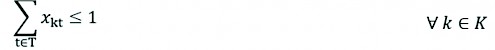
The objective function [1] is to maximize the discounted value of harvest-revenues minus the discounted costs of road construction and transportation within the forest; transportation cost from the forest’s point of entry to the point of utilization is not included. The objective function is comprised of five summations. The first summation in the objective function represents the total revenue from harvesting. The second summation represents the total discounted construction cost for the roads that cannot overlap. The third and fourth summations in the objective function represent the total discounted construction costs for the roads that can overlap. The fifth element of the objective function represents total transportation costs. The first constraint [2] ensures that a polygon may not be harvested more than once during the planning horizon. Equation [3] prevents the harvesting of polygons that are ineligible by age. The set of area-restricted adjacency constraints is defined in equation [4]. This is a standard formulation of area-restricted adjacency model (ARM), known as the path formulation, used by McDill et al. (2002) and Crowe et al. (2003). To use this equation, a set of maximum openings has been defined. Each maximum opening contains the minimal set of adjacent polygons that, if harvested together, would violate the maximum opening size limit.

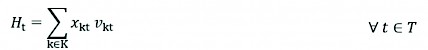
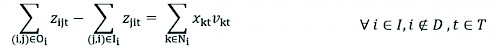
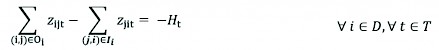
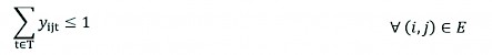
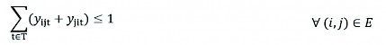
Equation [5] defines an accounting variable, Ht; the volume harvested in each period. Equation [6] uses this accounting variable to impose an upper bound on the volume that may be harvested in each period. The value of this upper bound is a parameter handed down from a strategic model and is used to ensure the long-term sustainability of the forest's multiple values. Equation [7] provides the link between the harvest scheduling activity and the network-flow model; i.e., if a polygon is cut, then the harvest volume is triggered to flow out of the node located in close proximity to this harvested polygon landing. If the polygon is not cut, then the node within that polygon may not function as a supply-node, but may function as a trans-shipment node. Equation [8] defines the demand-node, located at the entry-point of the forest. Equation [9] ensures that a road may be built only once during the planning horizon.

Equation [10] ensures that, if a flow of harvested wood passes from node i to j, then a road must be built along this arc, either in periods prior to the period of the flow, or in the period during which flow occurs–but not later. Equations [11] and [12] ensure that, if a road containing shared operational-scale arcs between nodes i and j is built, then all of the operational-scale nodes comprising this road must also be built.

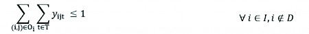
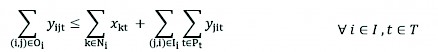
This formulation also contains the following strengthening constraints. Equation [13] strengthens the formulation by taking the form of a clique constraint. Klotz and Newman (2013) demonstrate the role of cliques in strengthening MIP formulations. In effect, [13] ensures that only one of the multiple possible roads exiting node i, may be built. This constraint makes sense because the volume harvested in a forest is typically transported by a truck; and when a truck enters a vertex within the road network, it will exit from one arc and cannot travel along two separate directed arcs. Equation [14] ensures that the potential of the flow of wood, along the same arc is constrained. Equation [15] is similar in structure to a »trigger« constraint first formulated by Kirby et al. (1986). Equation [15] ensures that, if a road is built at vertex j and enters vertex i, then a road exiting vertex i must be built in the same or prior periods. When [15] is combined with the clique constraint [13], then only one of the candidate roads exiting vertex i may be selected. Equation [16] ensures that, if a road is built exiting vertex i, then either: i) the polygon at vertex i must have been harvested; or ii) a road entering vertex i must have been built; or iii) both i) and ii). The distinction between [15] and [16] may be summarized as follows. For equation [15] the reasoning is: if a built road enters a vertex, then a road exiting that vertex must also be built. For [16] the reasoning is, if a road exits a vertex, then something must be responsible for its exiting that vertex: either a road entered it, or a polygon was cut, or both. Equation [17] is from Kirby et al. (1986). Due to its effectiveness, it has also been used by Guignard et al. (1998), Andalaft et al. (2003) and Veliz et al. (2015). Constraint [17] has also been referred to as a »trigger« constraint because it ensures that if a polygon is cut, then the construction of a road emanating from the vertex within that polygon is triggered to be built. The original integrated model already has the construction of a road triggered by a flow of wood passing through it (equation [10]) The construction of a road triggered by the harvesting of a polygon, from which a road emanates, has been shown to be computationally effective by Guignard et al. (1998) and Anadalaft et al. (2003). Equation [18] ensures that at least one of the roads leading to the forest's point of entry is built.

Finally, equations [19] and [20] constrain the harvest and road building decision variables to be binary, and equations [21], [22], [23] and [24] define the model’s continuous positive variables.

3. Case Study

The effects of including versus excluding transportation costs in the objective function of the integrated model were tested on three problem instances, derived from three forested areas within the Kenogami Forest Management Unit, located in the boreal forest of Ontario, Canada. All polygons, in each data-set, contain one of six yield curves, and the mean area of each polygon was 30 ha. Three problem instances, of different areas, were used: 6628, 12,622 and 19,677 ha and comprised of 244, 400 and 500 forested polygons, respectively. The maximum harvest opening restriction was 65 ha per period.

For each problem instance, the planning horizon was comprised of three five-year periods. The existing age-class distribution found in the case study was used. The minimum rotation age for each stand was set at 70 years. Revenue values of the standing timber were estimated using Armstrong's (2014) conversion return approach. Harvesting cost (i.e. the cost of felling, processing and extracting wood to the roadside), stumpage charges, reforestation and other management fees were deducted from the mill gate value of logs to calculate the revenue values before deducting road construction and transportation costs. These revenue values varied as a function of log diameter: $54 per m3 (ages 70 to 90 years), $62 per m3 (ages 91 to 120 years), and $70 per m3 (ages greater than 120). Transportation costs were estimated using the formulation in Martin (1971): assuming a truck load of 44 m3 and an average cost of $96 per hour for truck operation (private communication 2017), the marginal transportation cost inside the forest was estimated to be $0.30 per m3 per km. Both costs and revenues were discounted at 4% per annum, from the middle of each period. Adjacent polygons were defined as polygons sharing a common node.

The three forests were without a set of candidate roads. Therefore, a network of candidate roads was generated for each forest by using the optimal road location model of Anderson and Nelson (2004). This road location model allows one to generate an operationally feasible road, subject to vertical and horizontal design standards, that connects two points on a forested landscape at minimal cost. The optimal road location model was used with a 50×50 m grid layer (defining the scale of the operational-scale arcs) and a digital elevation model. All road design parameters, used in this work, were identical to those used by Anderson and Nelson (2004). The density of the entire set of candidate roads emerged from using the following rule: generate one candidate road connecting all pairs of adjacent forested polygons. In addition, all polygons adjacent to the forest's point of entry also had one road connecting them to this entry-point. The mean construction cost for all roads generated, for the three forests, was $35,377 per km with a standard deviation of $7940 per km. All currency units are Canadian dollars.

The number of decision variables required to solve the integrated harvest scheduling problem for these three forests over the three five-year periods is presented in Table 1.

Table 1 Dimensions of modeled problem instances, for three five-year periods

The integrated model was executed for a maximum of 3 hours on each problem instance, using the default search parameters in CPLEX® 12.5, on an Intel® Xeon X5650 hex-core processor, using 96 gigabytes of RAM, and a CentOS 5.5 operating system.

4. Results

The results are presented under four sub-headings: i) explanatory notes on the results; ii) general trend of the results; iii) the effect of problem size upon the results; and iv) the spatial attributes of the mapped solutions.

4.1 Explanatory Notes on Results

In Table 2, model A refers to the model with the objective function: maximize revenue – road construction costs – transportation costs; and model B refers to the model with the objective function: maximize revenue – road construction costs. Table 2 presents a comparison of the resulting objective function values, and their components, for each model. That is, Table 2 presents the resulting transportation costs that are entailed by the solutions of model B given the selected harvest blocks and the road network selected using model B. These entailed transportation costs were calculated from the flows of wood found in each of model B solutions, represented by the solution values for the flow variables, zijtand multiplying these values by the same marginal transportation cost ($0.30 per m3 per km) used in model A. Transport cost, in Table 2, is a measure ($ per m3) of the cost of moving harvested wood from the cut-blocks to the forest’s point of entry.

Table 2 Resulting solution attributes from applying the integrated model to three forests, using two different model A versus B

Second, the qualities of the solutions (i.e., proximity to the mathematical optimum) are presented in Table 2 under the column »Relative Gap«. Here we observe that: i) in none of the instances was the relative gap closed (after 3 hours of computing time); ii) the gaps ranged from 1.86% to 4.06%; and iii) the two different objective function values, for each forest, yielded solutions with very similar relative gaps, differing at most by 0.5%. Hence, based on the qualities of the solutions, it is reasonable to infer that the solutions are of sufficient quality to be quantitatively meaningful. Note: we do not here imply that any statistical inference is possible based on these results; for the sample size is too small. The results in this paper are, therefore, to be interpreted as illustrative.

4.2 General Trend of the Results

The general trend of the results in Table 2 are: i) no meaningful difference between harvest revenues and constructions costs can be observed between models A versus B; ii) major reductions in transportation costs can be observed in solutions, ranging from a reduction of 24.8% (for the smallest forest) to a reduction of 40.7% (for the largest forest); and iii) the reduction in total costs increased dramatically from 3.9% (for the smallest forest) to 21% (for the largest forest). From these trends, we observe that: i) the integration of transportation costs into the objective function yielded solutions with major reductions in both transportation and total cost of the tactical plan; and ii) as the total area of the forest tripled (from 6628 ha to 19,677 h) the percent reduction of in total costs that resulted from using model A versus B increased more than fivefold (from a 3.9% to 21%).

4.3 The Effect of Problem Size Upon the Results

The results in Table 2 indicate that the relative importance of transportation costs in the solutions increased as the size of the problem increased. In Table 3, this relative importance is represented as the ratio of transportation cost to revenue, and the ratio of transportation costs to construction costs, for each solution. These ratios are based on the data presented in Table 2.

Table 3 Ratios of revenue : transportation costs and of construction : transportation costs found in the solutions

The ratios in Table 3 show that, in the smallest forest, for every $1 spent on transportation, $55 in revenue was returned using model A, and $42 was returned using model B. In the largest forest, for every $1 spent on transportation, $17 in revenue was returned using model A and $10 was returned using model B. In other words, the influence of transportation costs upon the overall profitability of the solution did not remain constant as the size of the problem instance increased, but rather increased by a mean factor of 3.7 as the size of the forest approximately doubled in area. Similarly, Table 3 shows that, for the smallest forest, for every $1 spent on transportation, $7 were spent on road construction in model A and $5 were spent on road construction in model B. For the largest forest, for every $1 spent on transportation, $2 were spent on road construction in model A and $1 was spent on road construction in model B. In other words, (a) the relative importance of transportation costs increased as the problem size increased while the relative importance of construction costs decreased as the problem size increased; and (b) the influence of transportation costs upon the total costs of the solution increased by a mean factor of 4.25 as the area of the forest approximately doubled in area.

4.4 Mapped Solutions

Fig. 1a shows the mapped solution, for the 500 polygon forest, where transportation cost is included in the model’s objective function; and Fig. 1b shows the mapped solution where transportation cost is excluded. Table 2 shows that these two solutions generate almost similar values in revenues and in construction costs, but differ by 41% in transportation costs. These two maps show a set of spatial attributes worth noting.

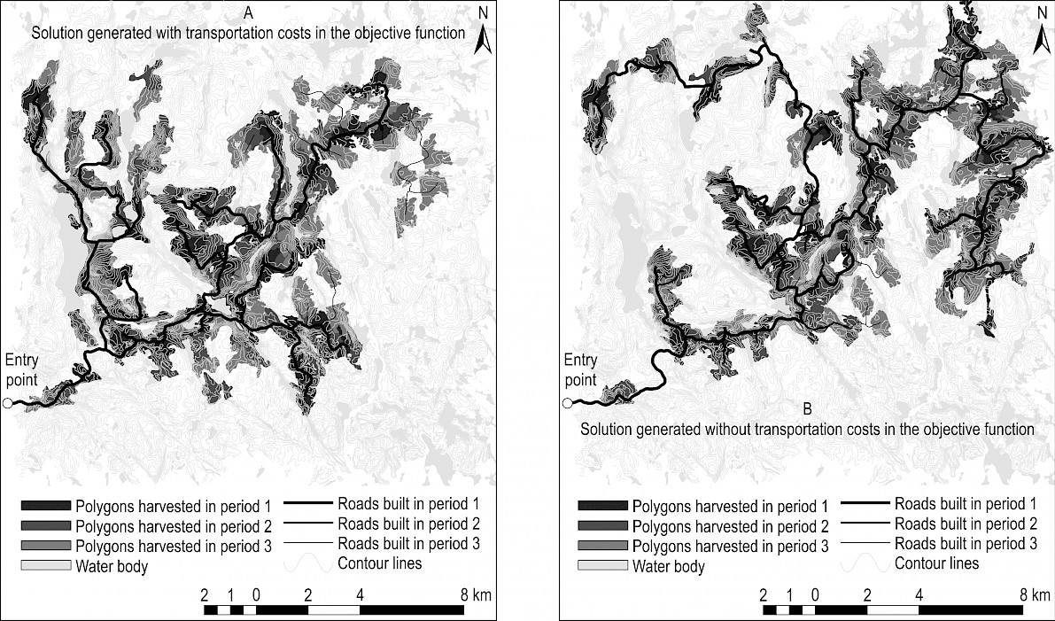
Fig. 1 Contour maps of two different solutions for the forest comprised of 500 polygons

Fig. 1 reveals that the solution produced using model B contains a set of harvest-blocks that are slightly more dispersed from the forest’s point of entry than does the solution generated using model A. This difference in spatial dispersion of harvest-blocks is not major, but it can be observed.

Fig. 1 also illustrates a trend for those polygons scheduled for harvest that are more remotely located from the point of entry. In Fig. 1b, the paths from these polygons to the point of entry are, in general, less than direct (i.e., more tortuous) than the paths from remote polygons in Fig. 1a.

Based on the two spatial attributes observed (dispersion of cut-blocks and directness of paths), it appears from Fig. 1 that the tortuous paths required to transport harvested wood from remote polygons to the point of entry are a greater cause of the increased transportation costs than the minor increase in dispersal of cut-blocks.

5. Discussion

The results of this work illustrate two interesting trends with regard to planning for transportation costs at the tactical level: i) that a model which simultaneously plans for harvest-revenue, and transportation and road-construction costs can consistently generate solutions with major reductions in transportation costs, when compared to a model which simultaneously plans only for harvest-revenue and road-construction costs; and ii) that the importance of planning for transportation costs increases greatly, relative to planning for construction, as the area of the forest increases. We will now discuss the implications of these results with regard to both forest management planning and research on tactical modeling.

As mentioned in the introduction, the appeal of metaheuristic algorithms to forest planners is that they can be used to solve large tactical planning models in a reasonable period of computing time. The disadvantage is that they have not, thus far, been adapted to solve models that plan simultaneously for: i) the location and timing of harvesting activities, ii) the construction of a road-network, and iii) the transportation of harvested wood through this road network. The results of this work suggest that this disadvantage can have a major economic impact upon the profitability of a forest management plan, and that this impact grows rapidly in magnitude as the size of the forest increases.

The economic significance of planning for transportation at the tactical scale should, therefore, influence research efforts directed at designing heuristic or metaheuristic algorithms that can be used to solve tactical planning models that integrate decisions on harvesting, road construction, and transportation activities. This research illustrates the merits of integrating all three of these decisions in one model.

6. Conclusion

In this work, an optimization model was built to provide mathematically optimal solutions for the tactical forest planning problem, where the objective function was to maximize revenue minus transportation and construction costs. The costs of transportation were either included in or excluded from the objective function as the model was applied to three forests of increasing size. The results indicate that the inclusion of transportation costs in the objective function has the effect of reducing both transportation costs and total costs; and that this reduction in costs increases as the size of the problems increases. The magnitude of the reduced costs also indicates that the problem of solving an integrated model, which includes transportation costs in the objective function, is of considerable economic importance, especially for large-scale forests. Hence, the results of this paper illustrate how the research problem of solving this problem is of a high economic priority in forest management planning.

Future research stemming from this work would include the development of a metaheuristic solution method that can be used to solve the integrated model on large-scale forests.

Acknowledgements

We thank NSERC strategic network on Value Chain Optimization (VCO), MITACS Canada, and aiTree Ltd. for funding this research. We also thank Tomislav Sapic for his generous assistance in using GIS. We acknowledge Waqas Ghouri, Timber Pricing Specialist and Tom Harries, Forest Industry Liaison Officer, from the Ontario Ministry of Natural Resources and Forestry (OMNRF) for sharing information about the parameters required to examine our model for this paper.

7. References

Andalaft, N., Andalaft, P., Guignard, M., Magendzo, A., Wainer, A., Weintraub, A., 2003: A Problem of Forest Harvesting and Road Building Solved through Model Strengthening and Lagrangean Relaxation. Operations Research 51(4): 613–628. https://doi.org/10.1287/opre.51.4.613.16107

Anderson, A.E., Nelson, J., 2004: Projecting vector-based road networks with a shortest path algorithm. Can. J. For. Res. 34(7): 1444–1457. https://doi.org/10.1139/x04-030

Armstrong, G.W., 2014: Considerations for boreal mixedwood silviculture: A view from the dismal science. For. Chron. 90(1): 44–49. https://doi.org/10.5558/tfc2014-009

Bettinger, P., Sessions, J., Johnson, K.N., 1998: Ensuring the Compatibility of Aquatic Habitat and Commodity Production Goals in Eastern Oregon with a Tabu Search Procedure. Forest Science 44(1): 96–112. https://doi.org/10.1093/forestscience/44.1.96

Bettinger, P., Chung, W., 2004: The Key Literature of, and Trends in, Forest-Level Management Planning in North America, 1950–2001. International Forestry Review 6(1): 40–50. https://doi.org/10.1505/ifor.6.1.40.32061

Bjørndal, T., Herrero, I., Newman, A., Romero, C., Weintraub, A., 2012: Operations research in the natural resource industry. Int. Trans. Oper. Res. 19(1–2): 39–62. https://doi.org/10.1111/j.1475-3995.2011.00800.x

Chung, W., Dykstra, D., Bower, F., O'Brien, S., Abt, R.M., Sessions, J., 2012: User's guide to SNAP for ArcGIS: ArcGIS interface for scheduling and network analysis program. USDA Forest Service PNW-GTR-847, 34 p.

Clark, M.M., Meller, R.D., McDonald, T.P., 2000: A three-stage heuristic for harvest scheduling with access road network development. For. Sci. 46(2): 204–218. https://doi.org/10.1093/forestscience/46.2.204

Crowe, K., Nelson, J.D., Boyland, M., 2003: Solving the area-restricted harvest-scheduling model using the branch and bound algorithm. Can. J. For. Res. 33(9): 1804–1814. https://doi.org/10.1139/x03-101

Goycoolea, M., Murray, A., Vielma, J.P., Weintraub, A., 2009: Evaluating Approaches for Solving the Area Restriction Model in Harvest Scheduling. Forest Science 55(2): 149–165. https://doi.org/10.1093/forestscience/55.2.149

Guignard, M., Ryu, C., Spielberg, K., 1998: Model tightening for integrated timber harvest and transportation planning. Eur. J. Oper. Res. 111(3): 448–460. https://doi.org/10.1016/S0377-2217(97)00362-7

Jones, J.G., Hyde, J.F.C., Meacham, M.L., 1986: Four analytical approaches for integrating land management and transportation planning on forest lands. Res. Pap. INT-36l, USDA Forest Service, Intermountain Research Station, Ogden, UT, 32 p.

Kirby, M.W., Wong, P., Hager, W.A., Huddleston, M.E., 1980: Guide to the integrated resource planning model. USDA Forest Service, Management Sciences Staff, Berkeley, Calif.

Kirby, M.W., Hager, W.A., Wong, P., 1986: Simultaneous planning of wildland management and transportation alternatives. TIMS Studies in the Management Sciences 21: 371–387.

Klotz, E., Newman, A.M., 2013: Practical guidelines for solving difficult mixed integer linear programs. Surveys in Operations Research and Management Science 18(1–2): 18–32. https://doi.org/10.1016/j.sorms.2012.12.001

Magnanti, T.L., Wong R.T., 1984: Network Design and Transportation Planning: Models and Algorithms. Transportation Science 18(1): 1–55. https://doi.org/10.1287/trsc.18.1.1

Martell, D.L., Gunn, E.A., Weintraub, A., 1998: Forest management challenges for operational researchers. European Journal of Operational Research 104(1): 1–17. https://doi.org/10.1016/S0377-2217(97)00329-9

Martin, J.A., 1971: The relative importance of factors that determine log-hauling costs. USDA Forest Service Research Paper NE-197. Northeastern Forest Experimental Station, Upper Darby, PA, 15 p.

McDill, M.E., Rebain, S.A. Braze, J., 2002: Harvest Scheduling with Area-Based Adjacency Constraints. Forest Science 48(4): 631–642. https://doi.org/10.1093/forestscience/48.4.631

Murray, A.T., 1999: Spatial Restrictions in Harvest Scheduling. Forest Science 45(1): 45–52. https://doi.org/10.1093/forestscience/45.1.45

Murray, A.T., Church, R.L., 1995: Heuristic solution approaches to operational forest planning problems. OR-Spektrum 17: 193–203. https://doi.org/10.1007/BF01719265

Naderializadeh, N., Crowe, K.A., 2018: Formulating the integrated forest harvest-scheduling model to reduce the cost of the road-networks. Operational Research, 1–24. https://doi.org/10.1007/s12351-018-0410-5

Nelson, J., Brodie, J.D., 1990: Comparison of a random search algorithm and mixed integer programming for solving area-based forest plans. Can. J. For. Res. 20(7): 934–942. https://doi.org/10.1139/x90-126

Richards, E.W., Gunn, E.A., 2000: A Model and Tabu Search Method to Optimize Stand Harvest and Road Construction Schedules. For. Sci. 46(2): 188–203. https://doi.org/10.1093/forestscience/46.2.188

Richards, E.W., Gunn, E.A., 2003: Tabu search design for difficult forest management optimization problems. Can. J. For. Res. 33(6): 1126–1133. https://doi.org/10.1139/x03-039

Silva, M.G., Weintraub, A., Romero, C., De la Maza, C., 2010: Forest Harvesting and Environmental Protection Based on the Goal Programming Approach. Forest Science 56(5): 460–472. https://doi.org/10.1093/forestscience/56.5.460

Veliz, F.B., Watson, J.P., Weintraub, A., Wets, R.B., Woodruff, D.L., 2015: Stochastic optimization models in forest planning: A progressive hedging solution approach. Annals of Operations Research 232(1): 259–274. https://doi.org/10.1007/s10479-014-1608-4

Weintraub, A., Navon, D., 1976: A Forest Management Planning Model Integrating Silvicultural and Transportation Activities. Management Science 22(12): 1299–1309. https://doi.org/10.1287/mnsc.22.12.1299

© 2019 by the authors. Submitted for possible open access publication under the
terms and conditions of the Creative Commons Attribution (CC BY) license (http://creativecommons.org/licenses/by/4.0/).

Authors’ addresses:

Nader Naderializadeh, PhD *

e-mail: nnaderia@lakeheadu.ca

Assoc. prof. Kevin A. Crowe, PhD

e-mail: kevin.crowe@lakeheadu.ca

Prof. Reino Pulkki, Dr. Sc. F.

e-mail: rpulkki@lakeheadu.ca

Lakehead University

Faculty of Natural Resources Management

955 Oliver Road, Thunder Bay

ON P7B 5E1

CANADA

* Corresponding author

Received: March 11, 2019

Accepted: December 02, 2019

Original scientific paper