Green Infrastructure Mapping in Urban Areas Using Sentinel-1 Imagery
doi: 10.5552/crojfe.2021.859
volume: 42, issue:
pp: 23
- Author(s):
-
- Gašparović Mateo
- Dobrinić Dino
- Article category:
- Original scientific paper
- Keywords:
- grey-level co-occurrence matrix (GLCM), land-cover classification, machine learning, speckle filtering, Synthetic Aperture Radar (SAR)
Abstract
HTML
High temporal resolution of synthetic aperture radar (SAR) imagery (e.g., Sentinel-1 (S1) imagery) creates new possibilities for monitoring green vegetation in urban areas and generating land-cover classification (LCC) maps. This research evaluates how different pre-processing steps of SAR imagery affect classification accuracy. Machine learning (ML) methods were applied in three different study areas: random forest (RF), support vector machine (SVM), and extreme gradient boosting (XGB). Since the presence of the speckle noise in radar imagery is inevitable, different adaptive filters were examined. Using the backscattering values of the S1 imagery, the SVM classifier achieved a mean overall accuracy (OA) of 63.14%, and a Kappa coefficient (Kappa) of 0.50. Using the SVM classifier with a Lee filter with a window size of 5×5 (Lee5) for speckle reduction, mean values of 73.86% and 0.64 for OA and Kappa were achieved, respectively. An additional increase in the LCC was obtained with texture features calculated from a grey-level co-occurrence matrix (GLCM). The highest classification accuracy obtained for the extracted GLCM texture features using the SVM classifier, and Lee5 filter was 78.32% and 0.69 for the mean OA and Kappa values, respectively. This study improved LCC with an evaluation of various radiometric and texture features and confirmed the ability to apply an SVM classifier. For the supervised classification, the SVM method outperformed the RF and XGB methods, although the highest computational time was needed for the SVM, whereas XGB performed the fastest. These results suggest pre-processing steps of the SAR imagery for green infrastructure mapping in urban areas. Future research should address the use of multitemporal SAR data along with the pre-processing steps and ML algorithms described in this research.
Green Infrastructure Mapping in Urban Areas Using Sentinel-1 Imagery
Mateo Gašparović, Dino Dobrinić
Abstract
High temporal resolution of synthetic aperture radar (SAR) imagery (e.g., Sentinel-1 (S1) imagery) creates new possibilities for monitoring green vegetation in urban areas and generating land-cover classification (LCC) maps. This research evaluates how different pre-processing steps of SAR imagery affect classification accuracy. Machine learning (ML) methods were applied in three different study areas: random forest (RF), support vector machine (SVM), and extreme gradient boosting (XGB). Since the presence of the speckle noise in radar imagery is inevitable, different adaptive filters were examined. Using the backscattering values of the S1 imagery, the SVM classifier achieved a mean overall accuracy (OA) of 63.14%, and a Kappa coefficient (Kappa) of 0.50. Using the SVM classifier with a Lee filter with a window size of 5×5 (Lee5) for speckle reduction, mean values of 73.86% and 0.64 for OA and Kappa were achieved, respectively. An additional increase in the LCC was obtained with texture features calculated from a grey-level co-occurrence matrix (GLCM). The highest classification accuracy obtained for the extracted GLCM texture features using the SVM classifier, and Lee5 filter was 78.32% and 0.69 for the mean OA and Kappa values, respectively. This study improved LCC with an evaluation of various radiometric and texture features and confirmed the ability to apply an SVM classifier. For the supervised classification, the SVM method outperformed the RF and XGB methods, although the highest computational time was needed for the SVM, whereas XGB performed the fastest. These results suggest pre-processing steps of the SAR imagery for green infrastructure mapping in urban areas. Future research should address the use of multitemporal SAR data along with the pre-processing steps and ML algorithms described in this research.
Keywords: grey-level co-occurrence matrix (GLCM), land-cover classification, machine learning, speckle filtering, Synthetic Aperture Radar (SAR)
1. Introduction
Forests are the most widely distributed terrestrial vegetation type, and thus play an important role in ecology and shaping the dynamics of regional and global ecosystem processes (Wulder 1998). The monitoring of green urban areas using remote sensing (RS) techniques can be used as a tool for integrated spatial planning (Gašparović and Dobrinić 2020). Moreover, using satellite imagery, urban areas with different characteristics and densities can be determined (Zhang et al. 2014). Benefits of green infrastructure (GI) in urban environments, such as mitigation of heat island effects and flood alleviation, are burdened by severe anthropogenic impacts that can diminish potential GI functionality. To counter that, the European Commission adopted the European Green Infrastructure Strategy, which aims to address the increasing fragmented nature of Europe urban areas as a result of human activities.
Optical satellite imagery is historically mostly used for monitoring the urban forest areas. As a result of easier interpretation and pre-processing methods, optical data is usually preferred to synthetic aperture radar (SAR) data. The optical RS system relies on the illumination of the Earth by the sun and measures the reflected radiation from a surface. Optical image quality can be seriously affected by atmospheric conditions (Jensen 2005). Active systems (like SAR) provide illumination by sending out microwaves and are mostly cloud independent. A radar system sends pulses of microwaves towards the Earth and records the intensity of the returned echoes for each pixel. Sentinel-1A (S1A), the first of the dual Sentinel-1 satellites, was launched in 2014 and has begun providing multi-temporal series of SAR imagery (C-band) at a time interval of 12 days. With Sentinel-1B (S1B), launched in 2016, the data provision has a repeat cycle of six days, while operating in a pre-programmed conflict-free mode (Veloso et al. 2017). Due to its all-weather, all-day imaging capability, several authors (Martinis et al. 2018, Twele et al. 2016) evaluated the possibility of the Sentinel-1 (S1) imagery for flood mapping or for irrigation mapping (Ferrant et al. 2017, Gao et al. 2018).
However, the single-use of SAR imagery for land-cover mapping has not been well-researched, partly as a result of the complexity, diversity, and availability of SAR data, and partly due to difficulties in data interpretation associated with speckle. Speckle noise, a common phenomenon in SAR systems, is associated to random interference between the coherent returns, and many filtering methods have been proposed, such as multi-looking, spatial filtering method, and transform domain filtering (Yuan et al. 2018). Idol et al. (2017) used the Lee-Sigma filter for radar speckle reduction on Radarsat-2 C-band imagery with a pixel resolution of 8 m. A maximum-likelihood decision rule was applied to create a classification map for four land cover classes. Overall accuracy (OA) for the despeckled radar imagery for both 3x3 and 5x5 window sizes was 60.3% and 62.2%, respectively. Maghsoudi et al. (2012) improved the classification results by applying speckle reduction on Radarsat-1 data and 7x7 enhanced Frost filter. Using a Bayes’ classifier to determine nine land-cover classes, OA was 60% for a single radar image.
Including texture information from the grey-level co-occurrence matrix (GLCM) can produce new images by making use of additional spatial information and different land-cover classes, which reflects in improving the classification accuracy. Balzter et al. (2015) investigated S1A imagery at 100 m spatial resolution for European CORINE land-cover mapping. Several random forest (RF) classifications of 27 land-cover classes were performed with different input bands. By using only horizontal-horizontal and horizontal-vertical backscatter values for the classification, OA, and Kappa values were 47.5% and 0.38, respectively. The highest classification accuracy of 68.4% and Kappa of 0.63 was achieved with auxiliary texture and geomorphometric input bands. Zakeri et al. (2017) used S1 and ALOS-2 PALSAR-2 imagery for land-cover classification (LCC) in Tehran. Using the backscattering values only on S1 imagery for the SVM classification of five land-cover classes, the OA was 45.70%, and Kappa was 0.30. In addition, texture features were selected from the PCA, and stacked with the backscattering polarised images. For SVM classification, the OA was increased to 54.25%, and Kappa to 0.41. Idol et al. (2017) added a variance texture measure created with the original Radarsat-2 image. Depending on the window size used for computing texture measure, OA ranged between 62.8% and 71.8%. Li et al. (2012) made a comparative analysis of ALOS PALSAR L-band and RADARSAT-2 C-band imagery. Different classification algorithms were examined for LCC on 10 classes in a tropical moist region. Classification accuracy on C-band data with maximum likelihood classifier achieved OA of 54.72% and Kappa of 0.42.
Most research focus only on speckle filtering of SAR imagery, or on extracting texture variables. This paper will evaluate how classification results change for S1 imagery during the classification of GI in urban areas on:
Þ original vertical-vertical (VV), vertical-horizontal (VH) bands
Þ speckled bands with different spatial filters
Þ GLCM texture features added to speckled image bands.
Furthermore, different machine learning methods were evaluated for the ability to produce LCC maps.
2. Materials and Methods
The objective of this study was to evaluate the use of single S1 imagery for land-cover mapping on three different study areas with an extent of 50×50 km. To reduce the speckle effect and to increase LCC accuracy, different adaptive filters were tested (Lee, refined Lee, Gamma-Map, and Lee-Sigma). Furthermore, VV and VH image texture were added along with speckled image bands, and the classification accuracy was compared. For this research, the machine learning (ML) methods used for land-cover mapping on the S1 imagery were random forest (RF), support vector machine (SVM), and extreme gradient boosting (XGB). Because of the high classification accuracy and their nonparametric nature, RF and SVM are mostly used for LCC (Noi and Kappas 2018, Rodriguez-Galiano et al. 2012), while the XGB classifier slightly outperformed RF and SVM in similar research (Man et al. 2018, Hirayama et al. 2019).

Fig. 1 Workflow of land-cover mapping used in this research
This paper is organised as follows (Fig. 1): (1) study area selection and data collection (see Section 2.1 and 2.2 for more details); (2) pre-processing of the SAR data, involving speckle noise filtering (SPK) and creation of the GLCM for deriving texture features (see Section 2.3 for more details); (3) land-cover classification using the RF, SVM, and XGB ML methods (see Section 2.4 for more details); and (4) evaluation to assess the classification accuracies obtained by the RF, SVM, and XGB (see Section 2.5 for more details).
2.1 Study Areas
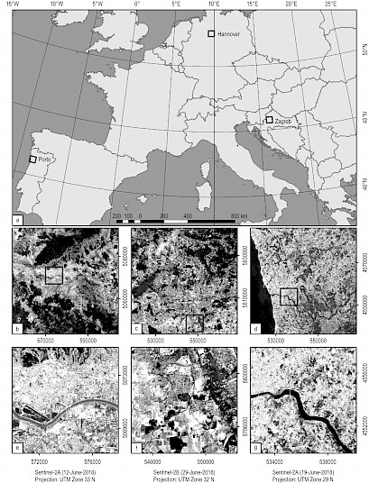
Fig. 2 (a) Study area locations; (b), (c), and (d) are entire study areas illustrated using a green band of Sentinel-2 (S2) imagery (band 3) with example subset locations (black square); (e), (f), and (g) are example subsets with an extent of 8×8 km for Zagreb, Hannover, and Porto
The land-cover mapping was applied to study areas across Europe with different geographical and environmental conditions (Fig. 2a), including the following towns: Zagreb in Croatia, Hannover in Germany, and Porto in Portugal. Zagreb (Fig. 2b) is surrounded by Medvednica mountain on the north and the Sava River on the south, and the rest represents a continental landscape with a uniform relief (Fig. 2e). Hannover (Fig. 2c)is the capital and largest city of the Federal State of Lower Saxony, Germany. The city is situated on the River Leine, and sometimes called the »garden city« for numerous parks, public gardens, and forests (Fig. 2f). Porto (Fig. 2d) is located in the northeast of the Iberian Peninsula and above the Douro River estuary. The city has a high population density and covers an area of approximately 45 km2 (Fig. 2g). The extent of the land-cover mapping in this research had the same dimensions (50×50 km).
2.2 Data
A polar-orbiting two-satellite S1 constellation was launched in 2014 (S1A) and 2016 (S1B). Both satellites carry a C-Band with the capability of providing dual polarisation observations in several measuring modes. The default mode over land is the interferometric wide-swath (IW) mode (Torres et al. 2012). S1 Ground Range Detected (GRD) products were acquired in the IW mode and used in this research. Level-1 GRD has been multi-looked and projected to the ground range. The characteristics of the used imagery and the acquisition dates are listed in Table 1.
Table 1 Characteristics of Sentinel-1 (S1) data used in this research
|
Zagreb |
Hannover |
Porto |
|
|
Acquisition date |
07-June-2018 |
09-July-2018 |
19-June-2018 |
|
Satellite |
S1A |
S1B |
S1A |
|
Acquisition orbit |
DESC |
ASC |
DESC |
|
Relative orbit |
124 |
66 |
125 |
|
Product Unique ID |
A9FA |
2500 |
B4D7 |
|
Pixel spacing |
10x10 m |
||
|
Polarisation |
VV, VH |
VV, VH |
VV, VH |
2.3 Pre-processing of SAR Data
Pre-processing steps of the S1 imagery were executed with the Graph Processing Tool (GPT) of ESA’s S1 Toolbox (S1TBX), which is embedded in the Sentinel Application Platform (SNAP, version 6.0). The GPT allows for consecutive execution of all individual pre-processing modules within a fully-automated processing chain (Twele et al. 2016). After applying an orbit file for precise orbit information, the SAR images must be radiometrically-corrected, terrain-corrected, and filtered due to the speckle noise. After pre-processing, each study area was cropped to the extent of 50×50 km. Visual analysis of classification maps were conducted for example subsets of 8×8 km.
Within the radiometric calibration, the pixel values of the images have to be transformed from radar reflectivity (stored as digital numbers) to a measure of the ground reflectivity or radar cross-section. The radiometric calibration is performed by calculating the sigma nought (σ0) or normalised radar cross-section coefficient. The source of the speckle noise is attributed to the random interference between the coherent returns. Image interpretation is difficult since the quality of the radar imagery is influenced by speckle. The speckle effect can be reduced using either multi-looking, filtering methods or transform domain filtering (Woodhouse 2006). In this research, several adaptive filters were evaluated using the SAR data. Filters are designed to adjust to local image variations to smooth the values and thereby reduce speckle, and lines and edges are enhanced to maintain the sharpness of the imagery. Based on previous studies (Hong et al. 2014, Kupidura 2016, Mansourpour et al. 2006), the filters used were Lee filters with window size 3×3 (Lee3), 5×5 (Lee5), refined Lee (RefLee), a Gamma-Map with window size 3×3 (Gamma3), and Lee sigma with window size 5×5 (LeeSigma5). Lee filter belongs to the local-statistics filter family, and smooths speckle in homogeneous areas, while details and high-frequency information are preserved in heterogeneous areas (Shi and Fung 1994). Many adaptive filters for speckle reduction have been developed on the basis of the Lee filter model (Ciuc et al. 2001).
Due to the terrain effects (foreshortening, layover, or shadowing effects), geometric distortions are not considered in the GRD imagery provided by ESA. Therefore, the GRD scenes have to be terrain-corrected from slant range to ground range geometry (Twele et al. 2016). One arcsecond Shuttle Radar Topography Mission (SRTM) digital elevation model (DEM) is used in this research. SRTM tiles are automatically downloaded by the S1TBX, and the S1 imagery is terrain-corrected. The images were projected in WGS 1984/UTM Zone 33 N (Zagreb), Zone 32 N (Hannover), and Zone 29 N (Porto). In the end, the σ0 coefficients were converted to dB using a logarithmic transformation (Zheng 2017):
 (1)
(1)
The ground surface texture within the image provides additional information regarding the land cover type that can be used for classification (Chand and Badarinath 2007, Masjedi et al. 2016). GLCM can be interpreted as joint grey level probability density distributions or 2-D image histograms. It characterises the texture parameters by calculating how often different combinations of pixel brightness with specific values and specified spatial relationships occur (Kuplich et al. 2005). Haralick et al. (1973) defined fourteen features that are calculated from this matrix. Principal component analysis (PCA) was used prior to classification for deriving the maximum possible information into the minimum additional texture information, which were then stacked with speckled input bands. In this research, the GLCM texture features – Mean (2), Contrast (3), and Variance (4) were calculated as follows (Zakeri et al. 2017):
 (2)
(2)
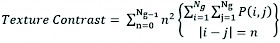 (3)
(3)
 (4)
(4)
Where:
pij (i,j) is the matrix cell index
R total sum of P
Px(i) which is equal to is the i-th entry in the matrix retreived by the row sums of p(i,j).
Prior to supervised classification, ten textural parameters were calculated from the original S1 imagery. In the research from Idol et al. (2017), higher classification results were obtained when texture measures were extracted from original S1 images than from despeckled imagery. After that, the first three components from the PCA result that contained the greatest variance of input variables were chosen (Fig. 3a, Fig. 3b, and Fig. 3c). The preliminary classification results in the Hannover area (Fig. 3d) are shown in Fig. 3e. With further investigation using various combinations of PCA components, it was decided to use the Mean, and the Variance as the input texture features for the GLCM classification (Fig. 3f).
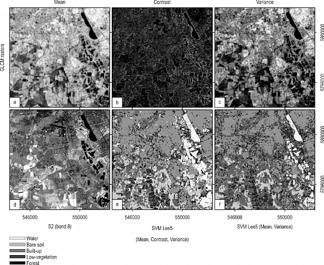
Fig. 3 Results of PCA for 8×8 km example subset in Hannover study area: (a) GLCM mean; (b) texture contrast; (c) GLCM variance; (d) study area illustrated using a near-infrared band of S2 imagery (band 8); (e) SVM classification with a Lee5 filter and three GLCM texture bands; (f) SVM classification with Lee5 filter and two GLCM texture bands
2.4 Machine Learning Methods for Land-Cover Classification
2.4.1 Random Forest
RF is an ensemble of a large number of tree-type classifiers, which are trained in parallel with bootstrapping followed by aggregation, jointly referred to as bagging. Bootstrapping reduces the overall variance of the RF classifier by using different subsets of available features in the model (Breiman 2001). Hence, some of the training samples will be chosen more than once, while some others will not be chosen at all in a new set. Essentially, random forest enables a large number of weak or weakly-correlated classifiers to form a strong classifier. For LCC, the RF algorithm is robust to the presence of mislabelled data, has high accuracy performance for large-scale study, and has easy-to-tune parameters (Pelletier et al. 2019).
2.4.2 Support Vector Machine
Like the RF, SVMs are also used for the production of land-cover maps through satellite image classification, due to their insensitivity to noise and overfitting of the data (Breiman 2001). The SVM was initially designed for binary (two-class) problems. To separate the two classes, the objective is to find an optimal hyperplane that represents the largest separation. The instances that rely on the margins are called support vectors, and by using them, the margin of the classifier is maximised (Cortes and Vapnik 1995). In this research, the classes might not be linearly separable. Kernel representations offer a solution in locating complex decision boundaries between classes. Different types of kernels can be used in the SVM classification: linear, polynomial, radial basis function (RBF), and sigmoid (Taati et al. 2015). According to Knorn et al. (2009), in LCC studies, the RBF kernel should provide the best overall results for GI mapping. When training an SVM with the RBF kernel, two parameters must be considered: the cost parameter (C) and the width of the kernel function named gamma (γ) (Qian et al. 2015). The C parameter decides the size of misclassification allowed for non-separable training data, and the γ parameter affects the smoothing of the shape of the class-dividing hyperplane (Noi and Kappas 2018). A large value of C may create an overfitted model, whereas adjusting the γ will influence the shape of the separating hyperplane.
2.4.3 Extreme Gradient Boosting
Extreme gradient boosting (XGBoost; XGB) is a regularised extension of traditional boosting ensemble techniques that belong to the classification and regression trees (CART) family of machine learning. As an ensemble tree-boosting method, the algorithm converts weak learners into strong learners (Georganos et al. 2018). Incorrectly classified samples receive higher weights at the next step, forcing the classifier to focus on their performance in the following iterations. The final classification is the most vigorous, as it includes the combined improvement of all the previously modeled trees (Chen and Guestrin 2016). Previously, gradient boosting models lacked a robust regularisation factor, making them susceptible to overfitting. In contrast, XGB overcomes this shortcoming by providing a stronger regularisation framework (Georganos et al. 2018).
2.5 Accuracy Assessment
For this study, the land-cover classes were selected following similar research and are shown in Table 2 (Gašparović and Jogun 2018, Gašparović et al. 2019). Polygons representing the aforementioned classes were chosen from Google Earth imagery, and from S2 satellite imagery acquired on similar dates as the S1 imagery for each study area. Following the examples of good practices for sampling design (Olofsson et al. 2014), stratified random sampling was applied to a single-date land-cover map. To classify the randomly-generated samples collected over the entire study area, the reference samples were divided into training (70%) and validation (30%) subsets (Table 2). In order to ensure the independence between the training and validation subsets, a separate probability sample for accuracy assessment was implemented (Stehman and Foody 2019).
Table 2 Overview of training and validation samples for each land-cover class
|
Zagreb |
Hannover |
Porto |
||||
|
Land-cover class |
Train. |
Valid. |
Train. |
Valid. |
Train. |
Valid. |
|
Water |
100 |
50 |
100 |
50 |
100 |
50 |
|
Bare soil |
200 |
100 |
200 |
100 |
200 |
100 |
|
Forest |
200 |
100 |
200 |
100 |
210 |
113 |
|
Built-up |
200 |
100 |
200 |
100 |
200 |
100 |
|
Low vegetation |
170 |
80 |
200 |
100 |
170 |
80 |
|
Total |
870 |
430 |
900 |
450 |
880 |
443 |
The classification accuracy was assessed using the Kappa coefficient (Kappa), and the overall accuracy (OA) (Congalton 1991). Furthermore, additional accuracy metrics, i.e., the user's accuracy (UA) and the producer's accuracy (PA), were derived from the confusion matrix. In such a way, the UA and PA are computed to represent individual class accuracies, instead of merely the OA accuracy. Training of the ML models and the accuracy assessment were conducted using the R programming language, version 3.4.1 (R Core Team, 2017).
3. Results
Overall, 11 classifications were computed for each study area. Classifications were computed for a radiometric classification on backscatter values (VV, VH); a radiometric classification on speckled VV, VH polarisations with different adaptive filters (SPK); and an integrated radiometric and texture feature classification with SPK polarisations (GLCM). Accuracy assessment for the pixel-based classifications was computed in terms of OA, Kappa, PA metrics, and UA metrics.
The highest classification results (Table 3) for VV, VH classification in Zagreb, Hannover and Porto was achieved by the SVM method, the OA was 65.70%, 61.79% and 61.92%, respectively. In the SPK classification in Zagreb, Hannover and Porto, the highest accuracy was achieved with the Lee5 filter with OA of 77.04%, 72.17% and 72.36% and using the SVM classifier, respectively. Classifications using GLCM features performed better than VV, VH and SPK in all test areas. For the GLCM classification, the highest accuracy in Zagreb, Hannover and Porto was obtained using a Lee5 filter with the SVM method, with OA values of 79.68%, 76.08% and 75.77%, respectively.
In all study areas, the SVM obtained higher accuracies than RF and XGB, with mean OA values for all classifications of 71.61%, 68.06%, and 69.15%, respectively (Table 3). Generally, the SPK classification achieved higher OA and Kappa values than radiometric classification on VV, VH polarisations. An additional increase in OA was obtained with the classification using GLCM texture bands. When comparing only GLCM results, the computed OA and Kappa values are similar, but the highest accuracies are achieved with the Lee5 filter.
Table 3 Overall accuracy (OA) and Kappa values of RF, SVM, and XGB, as applied to all three study areas
|
Zagreb |
Hannover |
Porto |
Mean values |
|||||||
|
Method |
OA, % |
Kappa |
OA, % |
Kappa |
OA, % |
Kappa |
OA, % |
Kappa |
||
|
Original |
VV, VH |
RF |
59.91 |
0.41 |
55.64 |
0.43 |
57.21 |
0.46 |
57.58 |
0.43 |
|
SVM |
65.70 |
0.48 |
61.79 |
0.49 |
61.92 |
0.52 |
63.14 |
0.50 |
||
|
XGB |
62.99 |
0.45 |
58.49 |
0.46 |
59.23 |
0.49 |
60.24 |
0.47 |
||
|
SPK |
Lee3 |
RF |
68.99 |
0.53 |
59.48 |
0.47 |
63.11 |
0.54 |
63.86 |
0.51 |
|
SVM |
72.30 |
0.57 |
67.23 |
0.56 |
68.10 |
0.60 |
69.21 |
0.58 |
||
|
XGB |
70.11 |
0.55 |
62.96 |
0.51 |
64.84 |
0.56 |
65.97 |
0.54 |
||
|
Lee5 |
RF |
74.39 |
0.61 |
66.00 |
0.56 |
68.39 |
0.60 |
69.60 |
0.59 |
|
|
SVM |
77.04 |
0.64 |
72.17 |
0.63 |
72.36 |
0.65 |
73.86 |
0.64 |
||
|
XGB |
74.92 |
0.62 |
67.13 |
0.57 |
69.34 |
0.61 |
70.46 |
0.60 |
||
|
RefLee |
RF |
60.02 |
0.42 |
55.60 |
0.43 |
57.30 |
0.46 |
57.64 |
0.44 |
|
|
SVM |
65.74 |
0.48 |
61.78 |
0.49 |
61.92 |
0.52 |
63.15 |
0.50 |
||
|
XGB |
62.80 |
0.45 |
58.49 |
0.46 |
59.29 |
0.49 |
60.19 |
0.47 |
||
|
Gamma3 |
RF |
69.09 |
0.53 |
59.51 |
0.47 |
63.07 |
0.53 |
63.89 |
0.51 |
|
|
SVM |
72.30 |
0.57 |
67.23 |
0.56 |
68.10 |
0.60 |
69.21 |
0.58 |
||
|
XGB |
70.11 |
0.55 |
62.96 |
0.51 |
64.98 |
0.56 |
66.02 |
0.54 |
||
|
LeeSigma5 |
RF |
59.97 |
0.41 |
55.63 |
0.43 |
57.30 |
0.46 |
57.63 |
0.43 |
|
|
SVM |
65.70 |
0.48 |
61.79 |
0.49 |
61.91 |
0.52 |
63.13 |
0.50 |
||
|
XGB |
62.99 |
0.45 |
58.49 |
0.46 |
59.31 |
0.49 |
60.26 |
0.47 |
||
|
GLCM |
Lee3 |
RF |
75.72 |
0.64 |
72.43 |
0.64 |
73.92 |
0.67 |
75.70 |
0.65 |
|
SVM |
78.97 |
0.68 |
75.04 |
0.67 |
74.81 |
0.68 |
77.35 |
0.68 |
||
|
XGB |
76.32 |
0.65 |
72.73 |
0.64 |
73.81 |
0.67 |
75.49 |
0.65 |
||
|
Lee5 |
RF |
76.45 |
0.65 |
73.47 |
0.65 |
74.81 |
0.68 |
76.24 |
0.66 |
|
|
SVM |
79.68 |
0.69 |
76.08 |
0.68 |
75.77 |
0.69 |
78.32 |
0.69 |
||
|
XGB |
76.75 |
0.65 |
73.98 |
0.66 |
74.11 |
0.67 |
76.22 |
0.66 |
||
|
RefLee |
RF |
75.53 |
0.64 |
71.65 |
0.63 |
73.33 |
0.66 |
75.44 |
0.64 |
|
|
SVM |
78.24 |
0.67 |
74.22 |
0.66 |
74.43 |
0.68 |
76.52 |
0.67 |
||
|
XGB |
76.09 |
0.64 |
71.67 |
0.63 |
73.11 |
0.66 |
75.15 |
0.64 |
||
|
Gamma3 |
RF |
75.75 |
0.64 |
72.48 |
0.64 |
74.11 |
0.67 |
75.72 |
0.65 |
|
|
SVM |
78.97 |
0.68 |
75.04 |
0.67 |
74.81 |
0.68 |
77.35 |
0.68 |
||
|
XGB |
76.32 |
0.65 |
72.73 |
0.64 |
73.80 |
0.67 |
75.44 |
0.65 |
||
|
LeeSigma5 |
RF |
75.54 |
0.64 |
71.88 |
0.63 |
73.44 |
0.67 |
75.30 |
0.65 |
|
|
SVM |
78.24 |
0.67 |
74.23 |
0.66 |
74.45 |
0.68 |
76.51 |
0.67 |
||
|
XGB |
76.21 |
0.64 |
71.67 |
0.63 |
73.03 |
0.66 |
75.22 |
0.64 |
||
The UA and PA accuracy metrics were used for the discrimination of the used land-cover classes. In Zagreb (Fig. 4), the UA and PA for the water class achieved the highest values using all three ML methods. Lower UA and PA values were achieved for the forest and built-up classes. The forest class yielded a higher UA than the built-up class, except for the SPK Lee5 classification with the SVM, and the built-up class achieved higher PA values. The lowest values of the UA and PA were achieved for bare soil and low vegetation. Regardless of the classification computed on VV, VH, SPK, or GLCM features, for the water class the UA value was in the range between 93.61% and 98.36%, and the PA value was in the range between 77.07% and 81.75%. Bare soil attained higher PA values than UA values, which means that the RF, SVM, and XGB methods correctly identified more ground truth pixels as bare soil, but the commission error for this class was much higher. This class was mostly misclassified as built-up. An increase of the UA from 79.03% on VV, VH to 86.76% with SPK, and additionally to 91.00% with GLCM was reported for the forest class. The built-up class was also well-classified, especially with the Lee5 filter for SPK and GLCM classifications with an SVM, where the UA values were 87.42% and 81.76%, respectively. The aforementioned filter also produced the highest PA values for the built-up class.
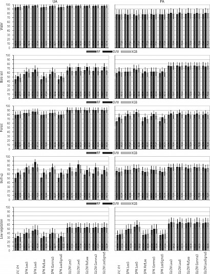
Fig. 4 UA and PA for the Zagreb study area (95% confidence level)
The lowest OA and PA values were obtained for the low vegetation class, as a result of a confusion between the forest and bare soil classes. The UA was in the range between 28.42% and 32.99% for classification on VV and VH; for SPK it was in the range between 28.35% and 48.49% and for the GLCM it was between 51.81% and 54.09%. Generally, the SVM classifier performed better than RF and XGB methods for all land-cover classes, except the forest class. For the forest class, the SVM had higher UA values for classifications on VV and VH, and on the SPK. Using the GLCM features, all three methods produced similar UA values for the forest class.
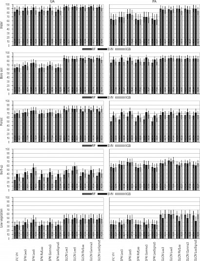
Fig. 5 UA and PA for Hannover study area (95% confidence level)
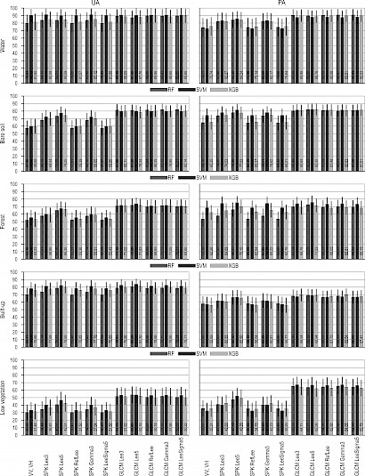
Fig. 6 UA and PA values for Porto study area (95% confidence level)
In Hannover (Fig. 5), all ML methods reached the highest UA for the water class in the range from 82.34% to 95.68%, and with lower PA values in the range between 62.54% and 90.07%. In Hannover, for the VV and VH and SPK classifications, the highest PA values were achieved in the bare soil class, in the range between 75.52% and 88.34%. Classification with texture bands (i.e., in the GLCM) increased the UA accuracy, especially for the bare soil class, with the highest difference of UA values between VV, VH, and GLCM classifications of 24.75%. The lowest UA values were achieved in the built-up and low vegetation classes. The UA values for the built-up class were in the range between 25.01% and 58.80%, and those for low vegetation were in the range between 30.59% and 50.49%. The built-up class yielded higher PA values than the low vegetation class. Built-up pixels were mostly misclassified as forest or low vegetation, whereas mostly low vegetation pixels were committed to the forest class. In Hannover, the SVM produced the highest UA values for the water, built-up, and low vegetation classes. For the VV, VH, and SPK classifications, the SVM classifier showed better performance for discrimination of the bare soil and forest class than the other two methods. However, for the bare soil class, the RF outperformed the SVM and XGB for the classification using the GLCM features, and for the forest class, both the RF and XGB methods achieved higher accuracy than the SVM.
In Porto (Fig. 6), the UA and PA values for the water class achieved the highest values for all three ML methods. The UA ranged between 79.80% and 91.30%, whereas the PA ranged between 73.07% and 90.97%. Slightly lower UA and PA values were achieved for the bare soil, and built-up classes, followed by the forest class, and the lowest UA and PA values were achieved for the low vegetation areas. The UA values for the bare soil class increased by approximately 11% between VV, VH, and SPK classifications using the RFmethod and Lee3 filter, and an additional 13% with additional texture bands (i.e., in the GLCM) stacked with Lee3 speckled polarisation. For the built-up class, the highest UA and PA values were achieved in Porto, as compared to Zagreb and Hannover, where the UA values were higher than PA values. This means that the omission error is much higher for this class. The UA values increased with the GLCM features for some land-cover classes (e.g., forest and low vegetation), meaning that the texture bands helped the ML methods to correctly separate these classes. The forest class achieved lower UA values than in Zagreb and Hannover because of confusion with the built-up and low vegetation classes. In this study area, the SVM achieved better UA results than the RF and XGB methods for all classes in the classifications on VV, VH, and SPK. All ML methods produced similar results in the classifications with the GLCM. Generally, the classification on a speckle filtered image with a Lee5 adaptive filter produced the best UA values for all classes, except for the water class, where Lee3 and Gamma3 produce better results. Additionally, stacked texture GLCM features improved the classification results for bare soil, forest, and low vegetation classes.
4. Discussion
This paper evaluates how different pre-processing steps of SAR imagery reflect on GI mapping in urban areas when applied to pixel-based classification. Compared to optical satellite data, SAR data has not been equally explored in GI urban applications due to its complexity. Three different ML methods (RF, SVM, and XGB) were applied to different study areas situated in Croatia, Germany, and Portugal (Fig. 1).
For the analysis of how classification accuracy changes during different pre-processing steps, classification was evaluated based on radiometric VV, VH backscatter values. The highest OA and Kappa (Table 3) were achieved with the SVM method, followed by XGB, while RF yielded the lowest accuracy. Therefore, our study confirmed the performance of these classifiers for LCC based on similar research (Noi and Kappas 2018, Dobrinić et al. 2020). The classification using single S1 imagery on VV, VH backscatter values with the SVM achieved a mean OA value of 63.14% and a Kappa of 0.50. The aforementioned results are similar to or slightly better than those obtained by Balzter et al. (2015) and Idol et al. (2017), who also used C-band SAR imagery for land-cover mapping. Since the salt-and-pepper effect is seen of LCC maps (Appendix A, Fig. A1–A3), an additional increase in classification results was done with speckle filtering. For speckle reduction, different adaptive filters were applied. Lee et al. (1994) have given a comprehensive review of the better-known SAR speckle filters, and based on that research, different adaptive filters were examined. Best classification results were obtained with Lee5 filter for all three ML methods – RF, SVM, and XGB, with OA of 69.60%, 73.86%, and 70.46%, respectively. Nevertheless, visually on LCC maps (Appendix A, Fig. A1–A3) salt-and-pepper effect is reduced and some land-cover classes (e.g., built-up, bare soil) are grouped together into thematic meaning. UA and PA metrics (Fig. 4, Fig. 5, and Fig. 6) prove that spatial filters improved the classification of the land-cover classes, especially forest, low vegetation, and bare soil class. In the SPK classification, a variability concerning the accuracy results among the study areas occurs, but the classification results have increased compared to the results obtained for the classification on original VV, VH bands. This positive trend in improving the classification results has been already reported by Maghsoudi et al. (2012), with an OA of 60% with 7x7 enhanced Frost filter. In research by Idol et al. (2017), a Lee-Sigma filter with 5x5 window was used for speckle filtering, and the obtained OA was 62.2%. Lv et al. (2015) evaluated land-cover classes in urban areas using RADARSAR-2 imagery. Using the SVM method, OA and Kappa of 76.79% and 0.74, were achieved, respectively. In this research, the highest OA and Kappa values were obtained with Lee filter. The aforementioned filter proved to be superior for visual and computational interpretation. It reduced misclassification between low vegetation and forest cover classes, and effectively preserved edges and features.
Since the SAR systems can distinguish textures, their use, as a measure of image roughness, proved to increase the classification accuracy for land-cover mapping (Balzter et al. 2015, Dekker 2001, Idol et al. 2017). In this research, the layer stacking of GLCM texture features (Mean and Variance) significantly increased the overall accuracy. The aforementioned texture bands were calculated from original VV, VH bands, and not on speckled bands, as reported in the paper by Idol et al. (2017). Speckle filtering reduces the capability of using texture features in LCC. The texture contrast was not included in the classification, as it showed significant noise in terms of enhancing the edges of objects to the water class (Fig. 2). A similar pattern occurs in the research by Zakeri et al. (2017), where the edges of different structures were recognised as a Built-up 3 class. Nevertheless, from the filter used and with the textural parameters, in this research, the mean OA yielded values for the SVM of 77.21%, followed by RF at 75.68%, while XGB yielded the lowest OA at 75.50%. A similar trend of increasing OA with adding texture bands to the classification was obtained by Balzter et al. (2015), who classified land-cover from S1 and SRTM DEM data using an RF classifier. The best result was achieved by adding GLCM measures and SRTM DEM data as input features, as the OA increased to 68.4%, and the Kappa was equal to 0.63. Idol et al. (2017) stacked variance texture measure to original VV, VH bands of RADARSAT-2 C-band imagery. The obtained classification accuracy for four land-cover classes was 72%. For the GLCM classification, visual improvement (Appendix A, Fig. A1–A3) can be seen, especially compared to VV, VH classification maps. The salt-and-pepper effect is reduced significantly, and a bigger agricultural fields (i.e., low vegetation class) or block of buildings can be recognised in GLCM classification maps.
Detailed insight of the land-cover classes are shown in Fig. 4, Fig. 5, and Fig. 6 for Zagreb, Hannover, and Porto through additional accuracy metrics (i.e., UA and PA), respectively. The water class achieved the highest UA for all three study areas. Due to its all-weather, all-day imaging capability, S1 imagery is mostly used for flood mapping (Amitrano et al. 2018, Martinis 2017). The forest class was also well-classified as reported in the research by Dostálová et al. (2018), where GLCM texture bands helped for better differentiation of this class. In the research by Zakeri et al. (2017), the UA value of 44.90% and the PA value of 65.20% for vegetation was obtained, whereas forest and low vegetation classes were discriminated more efficiently in this research. Slightly lower results were achieved for the bare soil class, wherein GLCM texture information increased the UA. The extraction of built-up areas was already investigated for S1 imagery by Pesaresi et al. (2016) and Zakeri et al. (2017). In this research, the built-up class was correctly identified in Zagreb and Porto, and the lowest UA accuracy was achieved in Hannover. Pesaresi et al. (2008) presented a procedure for the calculation of the texture-derived index for discrimination of the built-up structures. Their PanTex index reduces the edge effects and improves the capacity to distinguish between built-up and nonbuilt-up areas. In this research, the lowest OA and PA values were obtained in the low vegetation class, as a result of the confusion with the forest and bare soil classes. For better discrimination of the aforementioned land-cover class, multitemporal data (Gašparović and Dobrinić 2020) or integration with optical satellite data (Dobrinić et al. 2020) should be used. Furthermore, using cross-orbit (i.e., ascending and descending orbit), S1 imagery can improve land-cover type classification (Sayedain et al. 2020). In the aforementioned research, the accuracy results are at least 4% better than single-orbit classification. Therefore, the joint use of cross-orbit S1 imagery must be considered in the time-series analysis of the SAR imagery.
In this research, land-cover mapping was investigated for application in urban forest areas using single-date S1 imagery. The OA and Kappa values increased with speckle filtering, whereby Lee5 spatial filter performed the best among all filters used in this research. The highest classification accuracy was obtained with adding VV, VH image texture bands into the classification. Using PCA for selecting GLCM texture features prior to classification, produced higher classification results compared to similar research C-band data (Idol et al. 2017, Li et al. 2012, Zakeri et al. 2017). This research confirmed that using SPK (Lee5) and GLCM texture features (Mean and Variance) in urban areas are essential to modern urban planning and management, especially in combination with SVM classifier. Speckle filtering and additional input features (e.g., texture measures) improved LCC accuracy compared to previous research (Balzter et al. 2015, Clerici et al. 2017, Suresh et al. 2016). The main disadvantage of the aforementioned methods is the need for storage and processing capabilities to handle a large number of input features for classification. Therefore, feature selection methods (e.g., filter or wrapper methods) should be used for LCC (Tang et al. 2014). The aforementioned technique enables the ML algorithm to train faster, reduces overfitting, and improves the accuracy of a model (Inglada et al. 2016, Jin et al. 2018).
Future research is proposed using multitemporal radar data in order to better discriminate and classify GI in urban areas. Since results of this research cannot be directly compared to the classification made with optical data (e.g., S2), additional research should address the integration of radar and optical sensor data for LCC mapping, especially for areas mostly covered with clouds.
5. Conclusions
In this research, single-date S1 imagery was used as the data input for green infrastructure mapping of urban areas using three different ML methods (RF, SVM, and XGB). Due to the speckle noise inherent with radar, different adaptive filters were examined. In the final step, GLCM texture features as inputs were added along with speckled image bands, and the classification accuracy was compared.
The classification results, in terms of OA, increased by 14.51% from the classification on VV, VH polarisation to SPK classification with the Lee5 filter. The Lee5 filter obtained the highest classification results for speckle filtering. In addition, the textural parameters were calculated by applying a GLCM. Classification with GLCM texture bands, in terms of OA, increased 19.38% from the classification on VV and VH. The supervised classification results with texture features were found to be superior to the results without textures in two main aspects: higher accuracy and less noise. The highest improvement, in terms of UA and PA metrics, was achieved by low vegetation class, which can be additionally improved by the integration of the optical sensor data.
For the supervised classification of the urban forestry, the SVM method outperformed the RF and XGB methods. This study confirmed the efficiency of the SVM classifier for GI mapping in urban areas, which outperformed RF and XGB methods.
In order to produce accurate LCC maps in urban areas, pre-processing steps of SAR imagery described in this research, along with Lee5 spatial filter, GLCM texture bands (Mean and Variance) and SVM classifier should be used.
Acknowledgements
Support by the Croatian Science Foundation for the GEMINI project entitled: »Geospatial Monitoring of Green Infrastructure by Means of Terrestrial, Airborne and Satellite Imagery« (Grant No. HRZZ-IP-2016-06-5621) under which this research was conducted is gratefully acknowledged. We would like to thank the University of Zagreb that funded the RS4ENVIRO project entitled: »Advanced photogrammetry and remote sensing methods for environmental change monitoring« (Grant No. RS4ENVIRO) under which this research was conducted.
6. References Amitrano, D., Di Martino, G., Iodice, A., Riccio, D., Ruello, G., 2018: Unsupervised Rapid Flood Mapping Using Sentinel-1 GRD SAR Images. IEEE Transactions on Geoscience and Remote Sensing 56(6): 3290–3299. https://doi.org/10.1109/TGRS.2018.2797536
Balzter, H., Cole, B., Thiel, C., Schmullius, C., 2015: Mapping CORINE land cover from Sentinel-1A SAR and SRTM digital elevation model data using random forests. Remote Sensing 7(11): 14876–14898. https://doi.org/10.3390/rs71114876
Breiman, L., 2001: Random forests. Machine Learning 45(1): 5–32. https://doi.org/10.1023/A:1010933404324
Chand, T.R.K., Badarinath, K.V.S., 2007: Analysis of ENVISAT ASAR data for forest parameter retrieval and forest type classification – A case study over deciduous forests of central India. International Journal of Remote Sensing 28(22): 4985–4999. https://doi.org/10.1080/01431160701253295
Chen, T., Guestrin, C., 2016: XGBoost: A Scalable Tree Boosting System. In Proceedings of the 22nd ACM Sigkdd International Conference on Knowledge Discovery and Data Mining, San Francisco, California, USA, August 13–17, 785–794) p. https://doi.org/10.1145/2939672.2939785
Ciuc, M., Bolon, P., Trouvé, E., Buzuloiu, V., Rudant, J.P., 2001: Adaptive-neighborhood speckle removal in multitemporal synthetic aperture radar images. Applied Optics 40(32): 5954–5966. https://doi.org/10.1364/ao.40.005954
Clerici, N., Valbuena Calderón, C.A., Posada, J.M., 2017: Fusion of sentinel-1a and sentinel-2A data for land cover mapping: A case study in the lower Magdalena region, Colombia. Journal of Maps 13(2): 718–726. https://doi.org/10.1080/17445647.2017.1372316
Congalton, R.G., 1991: A review of assessing the accuracy of classifications of remotely sensed data. Remote Sensing of Environment 37(1): 35–46. https://doi.org/10.1016/0034-4257(91)90048-B
Cortes, C., Vapnik, V., 1995: Support-Vector Networks. Machine Learning 20(3): 273–297. https://doi.org/10.1023/A:1022627411411
Dekker, R.J., 2001: Texture analysis of urban areas in ERS SAR imagery for map updating. In IEEE/ISPRS Joint Workshop on Remote Sensing and Data Fusion over Urban Areas, DFUA 2001, 226–230 p. Institute of Electrical and Electronics Engineers Inc. https://doi.org/10.1109/DFUA.2001.985885
Dobrinić, D., Gašparović, M., Medak, D., 2020: Integration Of Multitemporal Sentinel-1 And Sentinel-2 Imagery For Land-Cover Classification Using Machine Learning Methods. In Proceedings of the International Archives of the Photogrammetry, Remote Sensing and Spatial Information Sciences (ISPRS), Nice, France, 14–20 June; XLIII-B1-2020, 91–98. p https://doi.org/10.5194/isprs-archives-XLIII-B1-2020-91-2020
Dostálová, A., Wagner, W., Milenković, M., Hollaus, M., 2018: Annual seasonality in Sentinel-1 signal for forest mapping and forest type classification. International Journal of Remote Sensing 39(21): 1–23. https://doi.org/10.1080/01431161.2018.1479788
Ferrant, S., Selles, A., Le Page, M., Herrault, P.-A., Pelletier, C., Al-Bitar, A., Mermoz, S., Gascoin, S., Bouvet, A., Saqalli, M., Dewandel, B., Caballero, Y., Ahmed, S., Maréchal, J.-C., Kerr, Y., 2017: Detection of irrigated crops from Sentinel-1 and Sentinel-2 data to estimate seasonal groundwater use in South India. Remote Sensing 9(11): 1119. https://doi.org/10.3390/rs9111119
Gao, Q., Zribi, M., Escorihuela, M.J., Baghdadi, N., Segui, P.Q., 2018: Irrigation mapping using Sentinel-1 time series at field scale. Remote Sensing 10(9): 1495. https://doi.org/10.3390/rs10091495
Gašparović, M., Jogun, T., 2018: The effect of fusing Sentinel-2 bands on land-cover classification. International Journal of Remote Sensing 39(3): 822–841. https://doi.org/10.1080/01431161.2017.1392640
Gašparović, M., Zrinjski, M., Gudelj, M., 2019: Automatic cost-effective method for land cover classification (ALCC). Computers, Environment and Urban Systems 76: 1–10. https://doi.org/10.1016/j.compenvurbsys.2019.03.001
Gašparović, M., Dobrinić, D., 2020: Comparative Assessment of Machine Learning Methods for Urban Vegetation Mapping Using Multitemporal Sentinel-1 Imagery. Remote Sensing 12(12): 1952. https://doi.org/10.3390/rs12121952
Georganos, S., Grippa, T., Vanhuysse, S., Lennert, M., Shimoni, M., Wolff, E., 2018: Very High Resolution Object-Based Land Use – Land Extreme Gradient Boosting. IEEE Geoscience and Remote Sensing Letters 15(4): 607–611. https://doi.org/10.1109/LGRS.2018.2803259
Haralick, R.M., Shanmugam, K., Dinstein, I., 1973: Textural Features for Image Classification. IEEE Transactions on Systems, Man, and Cybernetics SMC-3(6): 610–621. https://doi.org/10.1109/tsmc.1973.4309314
Hirayama, H., Sharma, R.C., Tomita, M., Hara, K., 2019: Evaluating multiple classifier system for the reduction of salt-and-pepper noise in the classification of very-high-resolution satellite images. International Journal of Remote Sensing 40(7): 2542–2557. https://doi.org/10.1080/01431161.2018.1528400
Hong, G., Zhang, A., Zhou, F., Brisco, B., 2014: Integration of optical and synthetic aperture radar (SAR) images to differentiate grassland and alfalfa in Prairie area. International Journal of Applied Earth Observation and Geoinformation 28(1): 12–19. https://doi.org/10.1016/j.jag.2013.10.003
Idol, T., Haack, B., Mahabir, R., 2017: Radar speckle reduction and derived texture measures for land cover/use classification: a case study. Geocarto International 32(1): 18–29. https://doi.org/10.1080/10106049.2015.1120356
Inglada, J., Vincent, A., Arias, M., Marais-Sicre, C., 2016: Improved early crop type identification by joint use of high temporal resolution SAR and optical image time series. Remote Sensing 8(5): 362. https://doi.org/10.3390/rs8050362
Jensen, J.R., 2005: Introductory digital image processing : a remote sensing perspective. (3th ed.). Prentice Hall, Upper Saddle River, USA.
Jin, Y., Liu, X., Chen, Y., Liang, X., 2018: Land-cover mapping using Random Forest classification and incorporating NDVI time-series and texture: a case study of central Shandong. International Journal of Remote Sensing 39(23): 8703–8723. https://doi.org/10.1080/01431161.2018.1490976
Knorn, J., Rabe, A., Radeloff, V.C., Kuemmerle, T., Kozak, J., Hostert, P., 2009: Land cover mapping of large areas using chain classification of neighboring Landsat satellite images. Remote Sensing of Environment 113(5): 957–964. https://doi.org/10.1016/J.RSE.2009.01.010
Kupidura, P., 2016: Comparison of filters dedicated to speckle suppression in SAR images. International Archives of the Photogrammetry, Remote Sensing and Spatial Information Sciences – ISPRS Archives 41: 269–276. https://doi.org/10.5194/isprsarchives-XLI-B7-269-2016
Kuplich, T.M., Curran, P.J., Atkinson, P.M., 2005: Relating SAR image texture to the biomass of regenerating tropical forests. International Journal of Remote Sensing 26(21): 4829–4854. https://doi.org/10.1080/01431160500239107
Lee, J.S., Jurkevich, I., Dewaele, P., Wambacq, P., Oosterlinck, A., 1994: Speckle filtering of synthetic aperture radar images: a review. Remote Sensing Reviews 8(4): 313–340. https://doi.org/10.1080/02757259409532206
Li, G., Lu, D., Moran, E., Dutra, L., Batistella, M., 2012: A comparative analysis of ALOS PALSAR L-band and RADARSAT-2 C-band data for land-cover classification in a tropical moist region. ISPRS Journal of Photogrammetry and Remote Sensing 70: 26–38. https://doi.org/10.1016/j.isprsjprs.2012.03.010
Lv, Q., Dou, Y., Niu, X., Xu, J., Xu, J., Xia, F., 2015: Urban land use and land cover classification using remotely sensed SAR data through deep belief networks. Journal of Sensors, 1–10 p. Article ID 538063 https://doi.org/10.1155/2015/538063
Maghsoudi, Y., Collins, M.J., Leckie, D., 2012: Speckle reduction for the forest mapping analysis of multi-temporal Radarsat-1 images. International Journal of Remote Sensing 33(5): 1349–1359. https://doi.org/10.1080/01431161.2011.568530
Man, C.D., Nguyen, T.T., Bui, H.Q., Lasko, K., Nguyen, T.N.T., 2018: Improvement of land-cover classification over frequently cloud-covered areas using landsat 8 time-series composites and an ensemble of supervised classifiers. International Journal of Remote Sensing 39(4): 1243–1255. https://doi.org/10.1080/01431161.2017.1399477
Mansourpour, M., Rajabi, M.A., Blais, J.A.R., 2006: Effects and Performance of Speckle Noise Reduction Filters on Active Radar and Sar Images. In Proceedings of ISPRS Ankara Workshop, Ankara, Turkey, 2006.
Martinis, S., 2017: Improving flood mapping in arid areas using SENTINEL-1 time series data. In 2017 IEEE International Geoscience and Remote Sensing Symposium (IGARSS), 193–196 p. IEEE. https://doi.org/10.1109/IGARSS.2017.8126927
Martinis, S., Plank, S., Ćwik, K., 2018: The use of Sentinel-1 time-series data to improve flood monitoring in arid areas. Remote Sensing 10(4): 583. https://doi.org/10.3390/rs10040583
Masjedi, A., Valadan Zoej, M.J., Maghsoudi, Y., 2016: Classification of Polarimetric SAR Images Based on Modeling Contextual Information and Using Texture Features. IEEE Transactions on Geoscience and Remote Sensing 54(2): 932–943. https://doi.org/10.1109/TGRS.2015.2469691
Noi, P.T., Kappas, M., 2018: Comparison of random forest, k-nearest neighbor, and support vector machine classifiers for land cover classification using sentinel-2 imagery. Sensors 18(1). https://doi.org/10.3390/s18010018
Olofsson, P., Foody, G.M., Herold, M., Stehman, S.V., Woodcock, C.E., Wulder, M.A., 2014: Good practices for estimating area and assessing accuracy of land change. Remote Sensing of Environment 148: 42–57. http://dx.doi.org/10.1016/j.rse.2014.02.015
Pelletier, C., Webb, G.I., Petitjean, F., 2019: Temporal Convolutional Neural Network for the Classification of Satellite Image Time Series. Remote Sensing 11(5): 523. https://doi.org/10.3390/rs11050523
Pesaresi, M., Corbane, C., Julea, A., Florczyk, A., Syrris, V., Soille, P., 2016: Assessment of the Added-Value of Sentinel-2 for Detecting Built-up Areas. Remote Sensing 8(4): 299. https://doi.org/10.3390/rs8040299
Pesaresi, M., Gerhardinger, A., Kayitakire, F., 2008: A Robust Built-Up Area Presence Index by Anisotropic Rotation-Invariant Textural Measure. IEEE Journal of Selected Topics in Applied Earth Observations and Remote Sensing 1(3): 180–192. https://doi.org/10.1109/JSTARS.2008.2002869
Qian, Y., Zhou, W., Yan, J., Li, W., Han, L., 2015: Comparing Machine Learning Classifiers for Object-Based Land Cover Classification Using Very High Resolution Imagery. Remote Sensing 7(1): 153–168. https://doi.org/10.3390/rs70100153
Rodriguez-Galiano, V.F., Ghimire, B., Rogan, J., Chica-Olmo, M., Rigol-Sanchez, J.P., 2012: An assessment of the effectiveness of a random forest classifier for land-cover classification. ISPRS Journal of Photogrammetry and Remote Sensing 67(1): 93–104. https://doi.org/10.1016/j.isprsjprs.2011.11.002
Sayedain, S.A., Maghsoudi, Y., Eini-Zinab, S., 2020: Assessing the use of cross-orbit Sentinel-1 images in land cover classification. International Journal of Remote Sensing 41(20): 7801-7819. https://doi.org/10.1080/01431161.2020.1763512
Shi, Z., Fung, K.B., 1994: Comparison of digital speckle filters. In International Geoscience and Remote Sensing Symposium (IGARSS) 4: 2129–2133. IEEE. https://doi.org/10.1109/igarss.1994.399671
Stehman, S.V., Foody, G.M., 2019: Key issues in rigorous accuracy assessment of land cover products. Remote Sensing of Environment 231: 111199. https://doi.org/10.1016/j.rse.2019.05.018
Suresh, G., Gehrke, R., Wiatr, T., Hovenbitzer, M., 2016: Synthetic aperture radar (SAR) based classifiers for land applications in Germany. International Archives of the Photogrammetry, Remote Sensing and Spatial Information Sciences – ISPRS Archives: 1187–1193. https://doi.org/10.5194/isprsarchives-XLI-B1-1187-2016
Taati, A., Sarmadian, F., Mousavi, A., 2015: Land Use Classification using Support Vector Machine and Maximum Likelihood Algorithms by Landsat 5 TM Images. Walailak Journal of Science and Technology 12(8): 681–687. https://doi.org/10.14456/WJST.2015.33
Tang, J., Alelyani, S., Liu, H., 2014: Feature selection for classification: A review. Data classification: Algorithms and applications: 37–64 p. https://doi.org/10.1201/b17320
Torres, R., Snoeij, P., Geudtner, D., Bibby, D., Davidson, M., Attema, E., Potin, P., Rommen, B.,Floury, B., Brown, M., Navas Traver, I., Deghaye, P., Duesmann, B.,Rosich, B., Miranda, N., Bruno, C., L'Abbate, M., Croci, R., Pietropaolo, A., Huchler, M., Rostanc, F., 2012: GMES Sentinel-1 mission. Remote Sensing of Environment 120: 9–24. https://doi.org/10.1016/j.rse.2011.05.028
Twele, A., Cao, W., Plank, S., Martinis, S., 2016: Sentinel-1-based flood mapping: a fully automated processing chain. International Journal of Remote Sensing 37(13): 2990–3004. https://doi.org/10.1080/01431161.2016.1192304
Veloso, A., Mermoz, S., Bouvet, A., Le Toan, T., Planells, M., Dejoux, J.F., Ceschia, E., 2017: Understanding the temporal behavior of crops using Sentinel-1 and Sentinel-2-like data for agricultural applications. Remote Sensing of Environment 199: 415–426. https://doi.org/10.1016/j.rse.2017.07.015
Woodhouse, I.H., 2006: Introduction to microwave remote sensing. CRC Press Taylor & Francis Group: Boca Raton, FL, USA.
Wulder, M., 1998: Optical remote-sensing techniques for the assessment of forest inventory and biophysical parameters. Progress in Physical Geography 22(4): 449-476. https://doi.org/10.1177/030913339802200402
Yuan, J., Lv, X., Li, R., 2018: A speckle filtering method based on hypothesis testing for time-series SAR images. Remote Sensing 10(9): 1383. https://doi.org/10.3390/rs10091383
Zakeri, H., Yamazaki, F., Liu, W., 2017: Texture Analysis and Land Cover Classification of Tehran Using Polarimetric Synthetic Aperture Radar Imagery. Applied Sciences 7(5): 452. https://doi.org/10.3390/app7050452
Zhang, J., Li, P., Wang, J., 2014: Urban Built-Up Area Extraction From Landsat TM/ETM+ Images Using Spectral Information And Multivariate Texture. Remote Sensing 6: 7339-7359. https://doi.org/10.3390/rs6087339
Zheng, Q., 2017: Satellite SAR Detection of Sub-Mesoscale Ocean Dynamic Processes (Vol. 44). World Scientific, London. https://doi.org/10.1142/9917
Appendix A
Hereinafter, visual assessments of LCC maps on VV, VH, SPK, and GLCM texture bands for Zagreb, Hannover, and Porto are shown in Fig. A.1, Fig. A.2, and Fig. A.3, respectively. The classification maps were computed with the RF, SVM, and XGB methods, and the extent of example subset is 8×8 km.
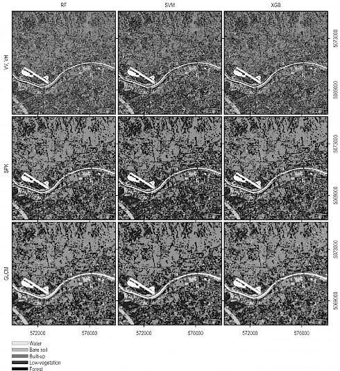
Fig. A1 Classification maps of land-cover on example subset using RF, SVM, and XGB on VV and VH polarisations; SPK with Lee5 filter; and GLCM texture features stacked with Lee5-filtered VV, VH polarisations for Zagreb study area
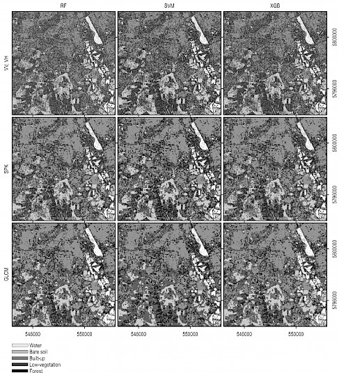
Fig. A2 Classification maps of land-cover on example subset using RF, SVM, and XGB on VV and VH polarisations; SPK with Lee5 filter; and GLCM texture features stacked with Lee5-filtered VV, VH polarisations for Hannover study area
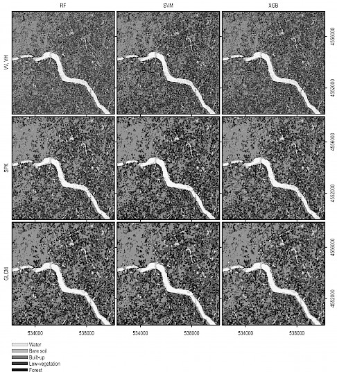
Fig. A3 Classification maps of land-cover on an example subset using RF, SVM, and XGB on VV and VH polarisations; SPK with Lee5 filter; and GLCM texture features stacked with Lee5-filtered VV, VH polarisation for Porto study area
© 2021 by the authors. Submitted for possible open access publication under the
terms and conditions of the Creative Commons Attribution (CC BY) license (http://creativecommons.org/licenses/by/4.0/).
Authors’ addresses:
Assist. prof. Mateo Gašparović, PhD *
e-mail: mgasparovic@geof.unizg.hr
Dino Dobrinić, MSc
e-mail: ddobrinic@geof.unizg.hr
Chair of Forest Inventory and Management
Faculty of Geodesy, University of Zagreb
Kačićeva 26
Zagreb
CROATIA
* Corresponding author
Received: March 16, 2020
Accepted: October 02, 2020
Original scientific paper