An Automated Approach for Extracting Forest Inventory Data from Individual Trees Using a Handheld Mobile Laser Scanner

Many dendrometric parameters have been estimated by light detection and ranging (LiDAR) technology over the last two decades. Handheld mobile laser scanning (HMLS), in particular, has come into prominence as a cost-effective data collection method for forest inventories. However, most pilot studies were performed in domesticated landscapes, where the environmental settings were far from those presented by (near)natural forest ecosystems. Besides, these studies consisted of numerous data processing steps, which were challenging when employed by manual means. Here we present an automated approach for deriving key inventory data using the HMLS method in natural forest areas. To this end, many algorithms (e.g., cylinder/circle/ellipse fitting) and machine learning models (e.g., random forest classifier) were used in the data processing stage for estimation of the tree diameter at breast height (DBH) and the number of trees. The estimates were then compared against the reference data obtained by field measurements from six forest sample plots. The results showed that correlations between the estimated and reference DBHs were very strong at the plot level (r=0.83–0.99, p<0.05). The average RMSE for tree DBHs was 1.8 cm at the forest landscape level. As for tree detection, 92.5% of 292 trunks were correctly classified on point cloud data. In general, estimation accuracy was sufficient for operational forest inventory needs. However, they could markedly decrease in »hard plots« located at rocky terrains with dense undergrowth and irregular trunks. We concluded that area-based forest inventories might hugely benefit from the HMLS method, particularly in »easy plots«. By improving the algorithmic performances, the accuracy levels can be further increased by future research.

An Automated Approach for Extracting Forest Inventory Data from Individual Trees Using a Handheld Mobile Laser Scanner

Mustafa Zeybek, Can Vatandaşlar

Abstract

Many dendrometric parameters have been estimated by light detection and ranging (LiDAR) technology over the last two decades. Handheld mobile laser scanning (HMLS), in particular, has come into prominence as a cost-effective data collection method for forest inventories. However, most pilot studies were performed in domesticated landscapes, where the environmental settings were far from those presented by (near)natural forest ecosystems. Besides, these studies consisted of numerous data processing steps, which were challenging when employed by manual means. Here we present an automated approach for deriving key inventory data using the HMLS method in natural forest areas. To this end, many algorithms (e.g., cylinder/circle/ellipse fitting) and machine learning models (e.g., random forest classifier) were used in the data processing stage for estimation of the tree diameter at breast height (DBH) and the number of trees. The estimates were then compared against the reference data obtained by field measurements from six forest sample plots. The results showed that correlations between the estimated and reference DBHs were very strong at the plot level (r=0.83–0.99, p<0.05). The average RMSE for tree DBHs was 1.8 cm at the forest landscape level. As for tree detection, 92.5% of 292 trunks were correctly classified on point cloud data. In general, estimation accuracy was sufficient for operational forest inventory needs. However, they could markedly decrease in »hard plots« located at rocky terrains with dense undergrowth and irregular trunks. We concluded that area-based forest inventories might hugely benefit from the HMLS method, particularly in »easy plots«. By improving the algorithmic performances, the accuracy levels can be further increased by future research.

Keywords: simultaneous localization and mapping (SLAM), light detection and ranging (LiDAR), mobile laser scanning (MLS), single-tree attributes, tree detection, forest inventory

1. Introduction

Forest management planning requires accurate and updated information for characterizing the current state of forest ecosystems. Periodical forest inventories are the primary data sources for this information flow (Kangas and Maltamo 2006, Ozkan and Demirel 2018). In inventory surveying, the number of trees and the diameter at breast height (DBH) are two essential parameters since they form the basis for both forest stand density and timber volume calculations (Wan et al. 2019). Unless having these data, neither the sustainable harvest rates nor the revenue of forest enterprises can be determined accurately (Bettinger et al. 2017, Bulut et al. 2016, Vatandaşlar and Zeybek 2020).

Conventional data collection methods (i.e., field measurements) are usually expensive, time-consuming, and labor-intensive in forest inventory surveying (Trotter et al. 1997). Therefore, remote sensing is widely used individually or combined with field measurements (Forsman et al. 2016, Gómez et al. 2019, Ozdemir and Karnieli 2011, Ucar et al. 2018). Laser scanners, in particular, are more common with the rapid development of light detection and ranging (LiDAR) technology worldwide (Balenović et al. 2019, Gómez et al. 2019, Hyyppa et al. 2008, Oveland et al. 2018, Valbuena et al. 2017, Wang et al. 2013). A comprehensive review, focused on different platforms of LiDAR (e.g., space-borne, airborne, terrestrial, etc.), can be seen in (Van Leeuwen and Nieuwenhuis 2010). Thanks to this technology, forest managers can quickly collect forest-related data on the ground at a reduced cost (Cabo et al. 2018, Del Perugia et al. 2019, Ryding et al. 2015).

Static LiDAR platforms have some limitations for operational forest inventory, such as the occlusion effect, low speed of data acquisition, and platform weight. Therefore, mobile laser scanners (MLS) have become preferable amongst forestry professionals recently (Bauwens et al. 2016, Hyyppa et al. 2020, Gollob et al. 2020). Given the carrier platforms, MLS can be grouped as: (i) vehicles, (ii), backpacks and (iii) handheld systems. The handheld mobile laser scanner (HMLS) systems, in particular, seem to be promising in forest inventories because the surveying time can be largely reduced thanks to their high mobility and lightweight (Balenović et al. (2021)). Indeed, one operator can collect data from trees at centimeter-level accuracy by simply walking through the forest with an HMLS at hand. Moreover, the dependency on GNSS has been eliminated in the latest systems, thanks to the Simultaneous Localization and Mapping (SLAM) algorithms. Thus, degraded GNSS signal under the canopy is no longer a problem in the forest. With the SLAM-based HMLS, point clouds can be automatically produced in the local coordinate system. Then, 3D data may be georeferenced to an absolute position. Readers are encouraged to see the compherensive study by Balenović et al. (2021) for more-detailed information on HMLS systems.

Using a SLAM-based HMLS, Gollob et al. (2020) successfully detected individual trees and estimated their DBHs in various forest conditions. They also used a density-based algorithm for the automatic detection of tree trunks. The researchers compared the HMLS-derived estimates with terrestrial laser scanner data and manual field measurements. In another study, Hyyppa et al. (2020) compared the accuracy of five LiDAR-based systems for operational forest inventory. They found that the HMLS and drone-mounted laser scanner (under-canopy) were superior to other systems for DBH and stem curve estimations. Similarly, Jurjević et al. (2020) estimated tree heights using HMLS and a drone-mounted laser scanner (over-canopy) in deciduous forest stands. The researchers compared the estimation results with traditional ground-based measurements. Their results showed a high level of agreement among the data sets. They stated that HMLS was a useful and reliable method for tree height measurement, especially for easy forest conditions in leaf-off season. More recently, Balenović et al. (2021) examined HMLS studies conducted in the forest inventory field. In this study, state-of-the-art applications of HMLS were reviewed, and the pros&cons of the method were documented in detail. They concluded that further research was needed to test the HMLS method potential for practical use in forest inventories.

Despite promising results from previous research (Bauwens et al. 2016, Giannetti et al. 2018, Gollob et al. 2020, Hyyppa et al. 2020), there is still a knowledge gap regarding the practical use of the HMLS, particularly in complex forest conditions. For instance, the extraction of individual tree parameters (post-processing) may still be challenging in dense and heterogenic plots located on poor sites. Researchers have examined different approaches (e.g., circle/cylinder fitting, etc.) to reach the best estimation accuracy for individual tree parameters derived by HMLS data (Koreň et al. 2017, Liu et al. 2018, Wu et al. 2018, Zhong et al. 2017, Zhou et al. 2019). Unfortunately, the accuracy requirements have not been fully met since trees generally show irregular morphological elements, such as noncircular trunks and complex branches. Therefore, these elements are poorly modeled in HMLS-based forest inventories. Indeed, more robust approaches are needed for automatically classifying and extracting tree trunks in »hard forest plots«. In this regard, the use of machine learning classifiers with untested morphological models (e.g., ellipse fitting for DBH estimation of a noncircular tree trunk) may solve the problem. This approach can minimize the estimation errors encountered in the post-processing stage. Thus, it needs to be tested in unmanaged natural forests presenting a non-homogeneous structure (Gadow et al. 2012).

The aim of this study is to develop a new and automated approach for extracting the number of trees and tree DBH data from 3D point clouds captured by a GeoSLAM ZEB-REVO HMLS device. Data accuracy was assessed based on comparing the extracted information with field measurements. To this end, 292 trees were scanned on six forest sample plots in an unmanaged natural forest. Several algorithms and shape fitting methods (i.e., circle, ellipse, or cylinder) were examined for improving data accuracy. The proposed approach is expected to promote the automation process in digital forest inventories, as well as to enhance the algorithmic performance in the data processing. Thus, forest inventory surveying is likely to be more cost-effective, especially in the mountainous countries with (near)natural forests. This will allow field personnel to save more time and money.

2. Materials and Methods

2.1 Study Area and Data Acquisition

The study area comprised six forest sample plots located at Artvin Province in the northeastern part of Turkey (Fig. 1). Artvin is the most mountainous city in the country. It is also in Caucasus Biodiversity Hotspot; thus, it hosts one of the highest rates of ecosystem diversity (Manvelidze et al. 2009). The main tree species in the forest are Picea orientalis, Pinus sylvestris, and Abies nordmanniana, along with Quercus dschorochensis, Fagus orientalis, and Castanea sativa. The average annual rainfall was 753 mm, while the average air temperature was 12.4 oC in the period 1949–2018 (SMS 2019). Forest sample plots were designated in different shapes and sizes. Detailed information on each plot is given in Table 1. Field surveys were carried out on October 1 and 2, 2018. First, essential data for forest inventory (the number of trees, DBH, slope degree, etc.) were measured and recorded into inventory sheets according to the conventional ground measurement methods described in the national guidelines (GDF 2017). At this stage, the lower tree DBH threshold was taken as 8 cm following GDF (2017). In the next stage, forest sampling plots were scanned using the ZEB-REVO HMLS device. Scanning time was 2–3 mins for a typical forest plot with 400 m2 in size. The survey path was planned as a closed-loop, as suggested by Del Perugia et al. (2019). During surveying, the surveyor started to walk from the plot center to the border and turned back several times. The starting point was also the endpoint of the path. In this way, the same area was scanned multiple times resulting in an increased scanning alignment. Finally, scanned LAS data were recorded on a personal laptop as the zip file for data processing.

Fig. 1 (a) Location of study area; (b) sampling plots

Table 1 Characteristics of forest sampling plots

2.2 Instrumentation

The point cloud data was acquired with the ZEB-REVO HMLS device (Cadge 2016) (https://geoslam.com) (Fig. 2). The device consists of a 2D time-of-flight laser scanner, as well as an integrated inertial measurement unit (IMU) on its rotary engine. Thanks to the lightweight (less than 1 kg), it can be easily used by one person at hand during labor-intensive forestry surveys. Furthermore, SLAM technology allows for generating a map of its surroundings and bear itself properly within the map. Thus, the map comes with a relative coordinate system. As a result, almost all dendrometric parameters (e.g., height, DBH, timber volume, etc.) can be modeled via 3D reconstructions. Technical specifications for the ZEB-REVO HMLS are presented in Table 2.

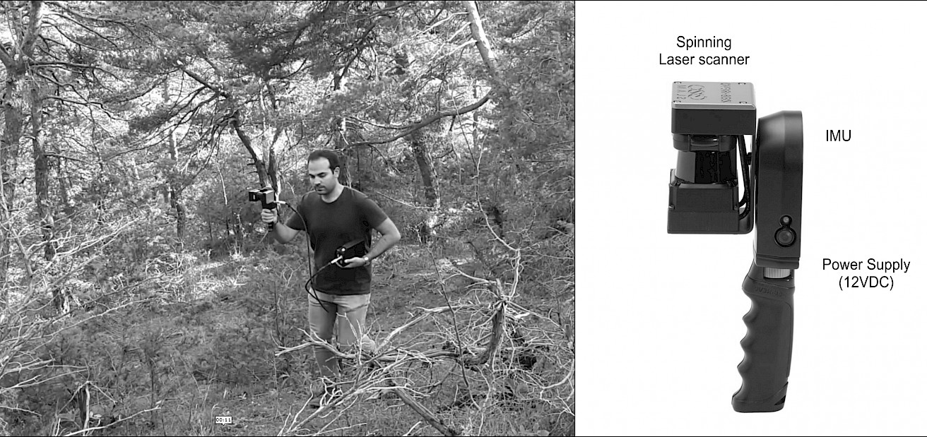
Fig. 2 Field data acquisition using ZEB-REVO HMLS device (https://geoslam.com)

Table 2 Specifications of ZEB-REVO HMLS

2.3 Methods

The methodology was mainly based on improving the estimation accuracy of dendrometric parameters collected by the ZEB-REVO HMLS using various algorithms. Then, the data were compared against the reference, conventionally measured on-the-ground. It should be noted that tree positions are unnecessary for most forest inventory studies since aggregated data are assessed at the plot-, stand-, or landscape levels. Therefore, only the plot centers were located using a handheld GPS, but individual trees were not registered into the real coordinate system. The general workflow can be seen in Fig. 3.

Fig. 3 Flowchart of the study

2.3.1 Pre-processing Stage

Raw data collected from the forest sample plots were pre-processed using GeoSLAM Hub desktop software (ZEB-REVO 2019). The SLAM algorithm was used to combine 2D coordinates with IMU data to generate 3D point clouds (ZEB-REVO 2019). The algorithm uses a method similar to the traverse technique (di Filippo et al. 2018) to convert raw data into point clouds. Unclassified point clouds were then clipped using the borders of forest sample plots based on coordinates of plot centers.

2.3.2 Data Processing and Modeling

As for ground/non-ground classification, the cloth simulation filtering (CSF) algorithm (Zhang et al. 2016) was implemented using the RCSF package in the R programming language (Roussel and Qi 2018). CSF uses a physical movement of the cloth model on the 3D point cloud. Optimal parameters were empirically tested for filtering. Accordingly, 0.2, 0.1, and 2.0 values were assigned for the class threshold, resolution, and rigidness parameters, respectively. These parameters may differ depending on landscapes because of the nature of the filtering algorithm. After filtering, points were classified as ground and non-ground in a LAS file.

As for normalization, an accurate digital terrain model (DTM) is essential. Tree heights are calculated based on DTM. To this end, DTM was created using the knnidw algorithm, which is a spatial interpolation method in the lidR package (Roussel and Auty 2019). It interpolates the ground points and creates a regularized DTM. Then, non-ground points were subtracted from the DTM using Eq. .

Where:

ZAGL distance from above ground points

ZNG above ground points

ZG ground points projected on DTM.

Finally, point cloud data were cross-sectioned between 1.0 and 2.0 meters above ground level (AGL). Thus, data density was reduced, and DBH estimations could be determined. However, some outliers might still exist in the cross-sections. Therefore, the statistical outlier removal (SOR) algorithm (Rusu 2010) was applied for noise reduction. Irregularities are another limitation along the tree trunks. In order to solve this problem, the moving least squares (MLS) algorithm and VoxelGrid up-sampling were implemented (Alexa et al. 2003). Graphical representation of the cross-sectioning stage (a.k.a. data slicing) can be seen in Fig. 4.

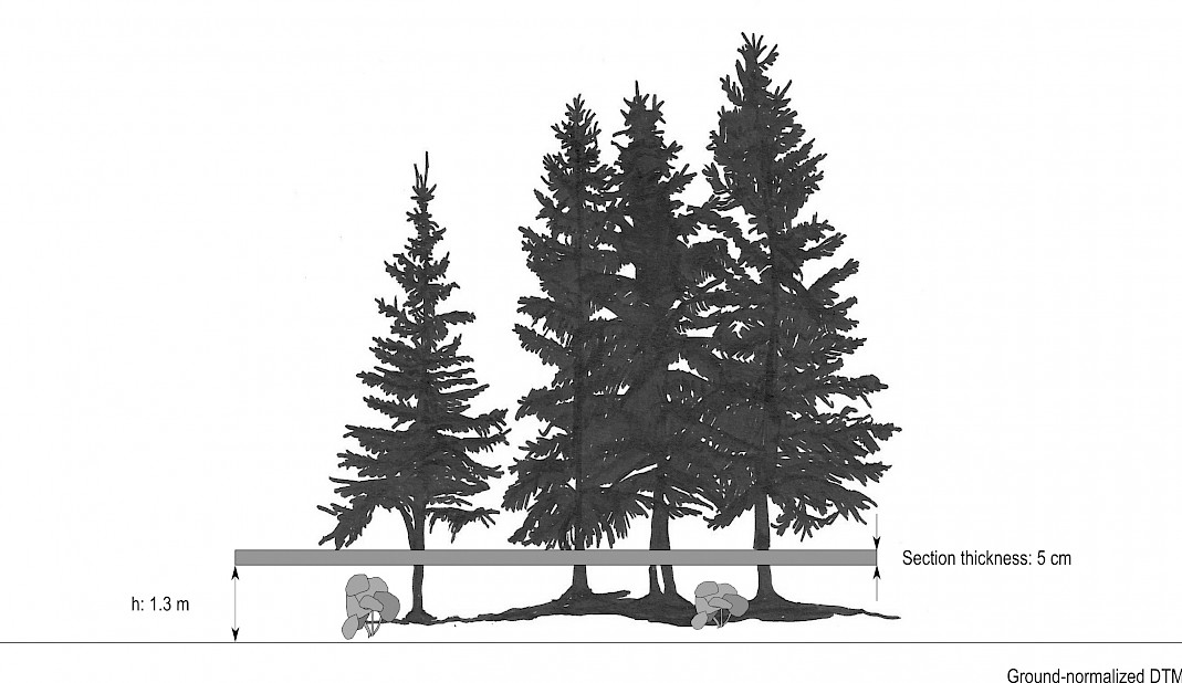
Fig. 4 Visualization of data slicing for generating cross-sections

2.3.3 Machine Learning Algorithm and Tree Extraction

After slicing the data, tree trunks need to be detected. This is a difficult task, particularly in complex forest plots with dense noise. The binary classification model, trained with Random Forest (RF) machine learning algorithm, can automatically detect trees within the point cloud data. In this way, tree DBH information can be extracted from classified data. It is a fundamental step for the automatic DBH estimation process.

To this end, the machine learning technique was performed based on geometric structures and the adjacency of point clouds. Thus, the points representing tree trunks were automatically extracted. Trunks were classified and labeled using the RF algorithm (Breiman 2001, Ni et al. 2017). For this, Caret package was used in the R programming language (Kuhn et al. 2019). In parallel, the local covariance matrix of an individual point was calculated using Eq. 2. After the calculation, eigenvalues were used as input elements.

(2)

Where:

pi given point in point cloud data

k point size of neighboor.

In the next step, surface normal and curvature, which are the two essential geometrical features, were estimated in the point cloud. The estimation of surface normal depends on the calculation of the approximate plane at each point position. The vector of the surface normal was then calculated from the eigenvectors and eigenvalues of the covariance matrix as described in (Montgomery et al. 2006). These elements allowed for clustering trunks, leaves, and branches from each other. Moreover, five different eigenvalue-based characteristics were used. These were omnivariance, planarity, linearity, surface variance, and anisotropy change (Ni et al. 2017). Regarding model accuracy, the k-fold cross-validation method was used for dividing data sets into k-subgroups. For this, the value of k was set to 10.

Finally, the Euclidean clustering extraction (ECE) algorithm (Rusu 2010) was applied for improving the fitting accuracy. Cluster analysis was used to classify and group a set of similar points that meet the threshold value in terms of distance. This approach, as a whole, was first applied to HMLS data for the forest inventory purpose.

2.3.4 Geometrical Shape Fitting

Given each cluster number, shape fitting is applied to the data that are separated as »tree« and »non-tree« trunks. Here, non-tree trunk points were excluded from the analysis in order to estimate tree DBHs robustly. For better DBH estimates, three morphological models, i.e., cylinder, circle and ellipse, were tested on each tree trunk. As for cylinder fitting, the analyses were performed in 1-m-thick sections between 1 m and 2 m AGL. For circle and ellipse fittings, 5-cm-thick sections were selected between 1.28 m and 1.33 m AGL (see Fig. 4).

The random sample consensus (RANSAC) technique was used for cylinder fitting (Nurunnabi et al. 2017, Schnabel et al. 2007). It was an iterative algorithm for estimating the parameters of a cylinder model. The maximum number of iterations was determined by Eq. (3):

(3)

Where:

N maximum number of iteration

p probability value in statistical test (taken as 0.99)

n minimum number of points for cylinder fitting

w probability for choosing an inlier.

CloudCompare RANSAC plugin was used for this process (Girardeau-Montaut 2019, Schnabel et al. 2007).

As for circle fitting, Izhak Bucher’s method (Bucher 1991) was used. The algorithm was developed in R programming language. The formula can be seen in Eq.

(4)

Where:

xc and yc coordinates for circle center

r circle radius

x and y coordinates for trunk points.

When Eq. is expanded using the parameters (a0, a1, a2), Eq. is obtained as follows:

(5)

Where:

a0=-2xc,

a1=-2yc,

a2=xc2+yc2-r2.

Circle parameters (xc, yc, r) were obtained by matrix solutions applied for trunk points.

Finally, the Conicfit package was used to ellipse fitting (Gama and Chernov 2015). The package uses Eq. (6) for fitting ellipse shape on trunk points:

(6)

Where:

k=(A,B,C,D,E,F)T the vector of parameters to be estimated.

The ellipse fitting method is also known as the orthogonal distance regression (ODR) (Al-Sharadqah and Chernov 2012, Gander et al. 1994). The ODR algorithm solves the minimization problem using Eq. .

(7)

Where:

diorthogonal distance from n data points ( ) to ellipse .

For decision-making between the ellipse and circle, the circle fitting method was first performed on each trunk data. Then, the distribution of distances to the center was calculated. Direction-dependent densities from the Y-axis were tested using a histogram. If the histogram is bimodal (see Fig. 5b), the first condition is met for the ellipse fitting. As for the second condition, the median absolute deviation (MAD) values are used. MAD is calculated based on the distances using Eq. (8):

(8)

Where:

c constant-coefficient used as 1.4826

x distance from center coordinates

median(x) centroid.

The threshold value for MAD was set to 3 in this study. However, it may vary depending on tree species in different forest settings. If the MAD value is higher than the threshold, then the second condition is met, and ellipse fitting is permanently chosen, as shown in Fig. 5c. Pseudo-codes used in the decision-making process can be seen in Algorithm 1. All the equations and algorithms presented in this subsection were written in the R programming language by the authors.

Algorithm 1 Decision-making procedure for using a circle or an ellipse fitting method

1: 2D point data P=x1, y1, ...xi, yi

Require: Circle fit to P 2: xc, yc ← P (Center)

3: n ← Peaks

4: if n < 2 then

5: Points are circle

6: else

7: Points are ellipse

8: end if

9: if MAD >= 3 then

10: Flag

11: end if

12: return Circle or Ellips

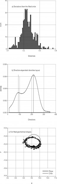
Fig. 5 Decision-making between circle and ellipse fitting methods

2.3.5 Accuracy Assessment and Correlation Analysis

Estimation accuracy was assessed both for machine learning classification and single-tree detection. As for machine learning, k-fold cross-validation (Lantz 2015) was performed. For this purpose, point cloud data was partitioned into two groups: training (70%) and test (30%) samples.

As for tree detection accuracy, a confusion matrix was generated. True positive, false positive, and false negative values were documented by visual interpretation for true detected, wrong detected, and undetected trees, respectively. Accordingly, recall, precision ratios, and F-scores were calculated using Eq (9)–(11):

(9)

(10)

(11)

Where:

r recall

p precision ratio

TP true positive

FP false positive

FN false negative.

Finally, scanned (estimation) and measured (reference) DBH data were subjected to Pearson’s correlation analysis. In this step, only TP trees were used against the reference data.

All these processes were implemented in R and C++ programming language (Gama and Chernov 2015, Kuhn et al. 2019, Roussel and Auty 2019, Rusu 2010, Team 2019) using a modest laptop with Intel Core i5-3210M (2.5 GHz) processor.

3. Results and Discussion

3.1 Individual Tree Detection and DBH Estimation

As for the number of trees estimations, it was found that F-scores from the six sampling plots differed between 0.78 and 1.0 with a mean of 0.93 (Table 3). The best estimation was obtained in Plot 2, which was a clean forest site with a canopy cover of about 50%. All trees were correctly detected on this plot. The plot had no undergrowth such as shrubs, seedlings or lying deadwoods on the forest floor. These kinds of elements often create noise on the point cloud, which may cause misclassifications. The worst estimation, on the other hand, was in Plot 4, in which almost half of the trees were wrongly detected (Fig. 6). This plot was on a poor site hosting many broadleaved trees on rocky terrain. The irregularities on low-quality trunks led to misclassified results. Similarly, Carr and Slyder (2018) found a mean F-score of 0.93 for a mixed temperate forest in Pennsylvania, USA. They stated that woody debris, dense shrub layer, and rough topography increased tree misclassifications, which was also the case in our study. Chen et al. (2019), on the other hand, correctly detected 93.3% of the tree trunks using a personal laser scanning device combined with SLAM technology in Beijing, China. It was seen that there was a good agreement for the individual tree detection (the number of trees) results obtained by the present study with those presented by other researchers. In another study by Gollob et al. (2020), tree stems in 20-m-radius circular plots were successfully mapped with a detection rate of 96%. The researchers stated that true detection rate was affected by plot size and the lower DBH threshold. The number of true detected trees generally increased with increasing threshold. In accordance with the national guidelines (GDF 2017), we only considered trees whose DBH≥8cm in the present study. It might be expected that if a higher threshold was taken, our F-scores could increase, too. In other words, the accuracy of HMLS-based tree detection is higher in mature forest stands than those of newly-developed or thin stands. This is also true for DBH estimates derived by HMLS data. Balenović et al. (2021) attributed this phenomena to: (i) high noise, (ii) low density of point clouds, (iii) low ranging accuracy, and (iv) high beam divergence provided by HMLS devices.

Table 3 Accuracy assessment for the number of trees parameter

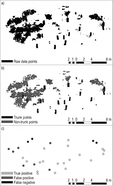
Fig. 6 (a) Perspective view of cross-sectioned raw data; (b) perspective view of data points classified by random forest model; (c) planar view of detected trunks

As for DBH, estimations were highly correlated with ground data in both cylinder and circle/ellipse fitting methods. Pearson’s r coefficients are given in Table 4. They were between 0.91 and 0.98 for cylinder fitting, and 0.83 and 0.99 for circle/ellipse fitting. Except for Plot 1, no statistically significant differences were found between cylinder and circle/ellipse fitting methods (p<0.05). In Plot 1, however, there were six forked trees (twins), which resulted in poor estimations, especially for the case of circle fitting. When necessary conditions were met, the ellipse fitting method provided more accurate estimates than circle fitting. The cylinder fitting method, on the other hand, took the cross-sections up to 2 meters, and thus, they could separately identify the forked trees. That was why its accuracy was higher than the circle/ellipse fitting in Plot 1. In the literature, there are different fitting methods applied to trees cross-sections. Gollob et al. (2020), for example, tried five different methods and stated that a natural cubic spline minimized the estimation errors for ZEB-REVO HORIZON HMLS data. For terrestrial laser scanner data, the best method was reported as ellipse fitting in the same study. They stated that small trees (DBH<10 cm) were generally overestimated, while large trees (>10 cm) were underestimated by HMLS regardless of the fitting method.

Table 4 Accuracy assessment for DBH parameter

In the present study, the best DBH estimations were made for Plot 3, where regular and high-quality spruce trunks existed. Their smooth barks may also help to obtain more accurate results. In contrast, the plots with mature Scots pine trunks, such as Plot 4 and Plot 5, yielded poorer estimates because of their thick and rough barks. Their bark structures frequently generated noises along the trunks on the point cloud data. Nevertheless, the results were generally in line with the related literature. Xi et al. (2016), for example, achieved an r coefficient of 0.98 between the estimated and field data, which was close to ours. Slight differences may stem from different tree species or distinct topographic settings.

The RMSEs in DBH estimations showed a relatively high variation from 0.7 to 4.9 cm with a mean of 1.8 cm in the circle/ellipse fitting method (Table 4). In the cylinder fitting method, contrastingly, they were more stable. However, its RMSEs were generally higher than those of circle/ellipse fitting. That was why the average RMSE for circle/ellipse fitting was 0.1 cm lower than the cylinder fitting method. Chen et al. (2019) and Xi et al. (2016) conducted similar LiDAR-based studies in China and Finland. They achieved the RMSEs of 1.58 and 0.90 cm, respectively. The lower values can be attributed to different instrumentations used in these studies. Xi et al. (2016), for example, used a TLS instrument (Leica HDS6100), while Chen et al. (2019) used personal laser scanning with a real-time viewer (ZEB-REVO RT). On the other hand, Balenović et al. (2021) recently reviewed the HMLS studies in the forestry literature. In this review, RMSEs were higher in the studies, including smaller trees (<10 cm) into the analyses. Accordingly, RMSEs ranged from 2.3 cm to 3.1 cm in the studies by Ryding et al. (2015), Oveland et al. (2018), and Gollob et al. (2020). In the present study, the lower DBH threshold was taken as 8 cm, as done in the Turkish forest management system.

Importantly, an assessment for bias is needed for reliable DBH estimations. Pearson’s r coefficients can be very high, even for heavily biased data. Therefore, bias values for DBH estimations are also presented in Table 4. They were 0.97 cm and −0.87 cm for cylinder and circle/ellipse fitting methods, respectively. The average values close to zero showed that DBH estimations were almost unbiased. At the plot level, however, relatively biased data were found in Plot 1 for both cylinder (2.63 cm) and circle/ellipse (−9.72 cm) methods. Hyyppa et al. (2020) estimated tree DBHs using HMLS in a forest type (pine+spruce+birch) similar to ours. They reported bias values as −0.39 cm and −0.44 cm for easy (sparse) and hard (obstructed) forest plots, respectively. The differences are attributable to the HMLS devices used by two studies. We used an older model of ZEB-REVO, which had a maximum outdoor range of ~15 m in practice. Hyyppa et al. (2020), on the other hand, used the newer model - ZEB-REVO HORIZON. The maximum range for ZEB-REVO HORIZON is reported as ~100 m in its user manual (https://geoslam.com).

3.2 Performance of Machine Learning Model

An RF algorithm was used for segmentation, training, and validation steps of the entire classification process. It was found that the surface normal at the Z-axis (nz), planarity, and omni-variance were three important features for the training of the model (Fig. 7). A total of 20,000 data points were used since additional points did not significantly improve the model accuracy according to Cohen’s kappa index. As seen in Fig. 8, the overall accuracy and kappa index rates were 96.06% and 88.8%, respectively. This classification accuracy is satisfactory for most forestry applications, as suggested by Kangas and Maltamo (2006) and Vatandaşlar and Zeybek (2020).

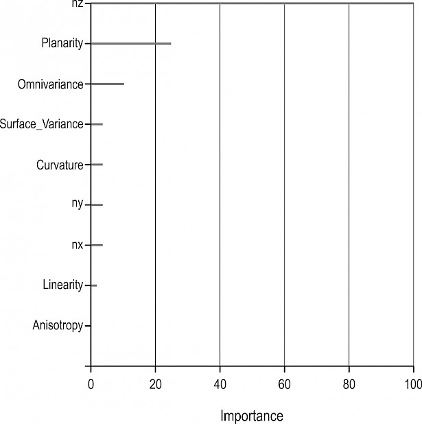
Fig. 7 Importance for variables of random forest model

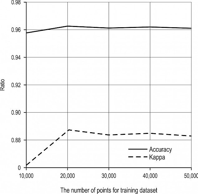
Fig. 8 Effect of number of data points on Random Forest’s training set

3.3 Further Improvements in Algorithmic Performance

For further improvements in algorithmic performance, the MLS method was applied to reduce point scattering on tree trunks. The result was satisfying, as clearly seen in Figs. 9a−b. The parameter set for polynomial order and point search radius was 2 cm and 0.05 cm, respectively. It was observed that 11% of the data points deviated from the projected surface within a limit of 1.5−3.0 cm. The main reason for the deviations is thought to be bark roughness and the precision of laser footprint. 85% of the data points, on the other hand, were within a limit of 0−1.0 cm distance from the surface (Fig. 9c). To overcome the point density problem, the up-sampling interval in MLS was taken as 1.0 cm for some trees. Moreover, neighborhood and standard deviation values for the SOR application were set to 3 and 1, respectively. As a result, an agreement of 99.9% was obtained between the field and enhanced data at the single-tree level.

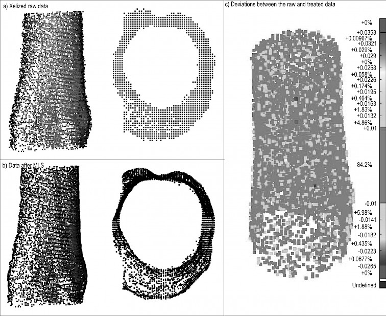
Fig. 9 Noise reduction on point clouds

The first step in the segmentation process is to cross-section the point cloud data. It is also known as data slicing, as graphically shown in Fig. 4. In fact, there is no consensus for an optimal slice thickness in the literature. Liu et al. (2018), for example, compared ten different values (from 1 to 10 cm) for circle fitting for oak, pine, and spruce species. They found 6-cm-thick slices were the best for minimizing the errors in DBH estimates. In their case, the average RMSE for tree DBHs was found to be 2.3 cm. In our case, 5-cm-thick slices yielded the best result with an RMSE range from 0.7 cm to 4.9 cm, depending on the sample plot characteristics.

As for the cylinder fitting, a thickness value of 1.0 m was applied between 1.0 m and 2.0 m AGL in the present study. Similarly as in the circle fitting, there is no optimal thickness value for the cylinder fitting method in the relevant studies. In a study conducted in China, Chen et al. (2019) proposed a thickness value of 40 cm between 1.1 m and 1.5 m AGL for the non-contact cylinders. Since there is considerable uncertainty in the forestry literature, future studies should focus on parameterization of the different tree species in this manner.

4. Conclusions

In this study, the ZEB-REVO HMLS was used to retrieve essential inventory data from the natural forest plots under harsh topographic conditions. A new approach was developed in the R programming language for fully-automating the data extraction process, which was manually done by commercial software before. Moreover, many algorithms were tested to minimize the classification error encountered during the tree detection stage.

The results showed that both the number of trees and tree DBH parameters could be estimated at acceptable accuracy levels. The data accuracy was generally more than 90%, which was enough for the plot-level forest inventories. It was also seen that the ellipse fitting method, in general, provided a more convenient solution for DBH estimations than the circle and cylinder fitting methods. However, the data accuracy significantly decreased in some »hard forest plots«. These plots had noisy elements, such as undergrowth vegetation, dense branches, forked trees, and microhabitats along tree trunks.

In conclusion, HMLS offers high operational potential for forest inventory surveying. Therefore, automated approaches - such as those presented in this study – will likely be more prevalent in the forestry sector. Thus, less field time and labor force are likely to be needed for forest professionals in the near future. However, the potential of HMLS should be further investigated in other forest types, presenting different stand structures and environmental settings. Likewise, the feasibility of HMLS should be tested for many applied fields of forest engineering, including forest road maintenance, silvicultural interventions, and logging operations.

Acknowledgments

This research did not receive any specific grant from funding agencies. Nevertheless, the authors would like to thank Mehmet Kocamanoğlu, the general manager of Geomatics Group, for providing the ZEB-REVO HMLS device. The authors are also grateful to Melih Ergün and Onur Şahin, the Geomatics Group’s engineers, for their assistance in the field.

5. References

Al-Sharadqah, A., Chernov, N., 2012: A doubly optimal ellipse fit. Comput. Stat. Data An. 56(9): 2771–2781. https://doi.org/10.1016/j.csda.2012.02.028

Alexa, M., Behr, J., Cohen-Or, D., Fleishman, S., Levin, D., Silva, C.T., 2003: Computing and rendering point set surfaces. IEEE Trans. Vis. Comput. Graph. 9(1): 3–15. https://doi.org/10.1109/Tvcg.2003.1175093

Balenović, I., Jurjević, L., Milas, A.Š., Gašparović, M., Ivanković, D., Seletković, A., 2019: Testing the applicability of the official Croatian DTM for normalization of UAV-based DSMs and plot-level tree height estimations in lowland forests. Croat. J. For. Eng. 40(1): 163–174.

Balenović, I., Liang, X., Jurjević, L., Hyyppä, J., Seletković, A., Kukko, A., 2021: Hand-held personal laser scanning–current status and perspectives for forest inventory application. Croat. J. For. Eng. 42(1): 165–183. https://doi.org/10.5552/crojfe.2021.858

Bauwens, S., Bartholomeus, H., Calders, K., Lejeune, P., 2016: Forest inventory with terrestrial LiDAR: A comparison of static and hand-held mobile laser scanning. Forests 7(12): 127. https://doi.org/10.3390/f7060127

Bettinger, P., Boston, K., Siry, J.P., Grebner, D.L., 2017: Forest Management and Planning, Academic press, 362.

Breiman, L., 2001: Random forests. Mach. Learn. 45(1): 5–32. https://doi.org/10.1023/A:1010933404324

Bucher, I., Circle fit. Available online http://www.mathworks.com/matlabcentral/fileexchange/5557-circle-fit/content/circfit.m (accessed 8 December 2020)

Bulut, S., Günlü, A., Keleş, S., 2016: Estimation of some stand parameters using Göktürk-2 satellite image. In Forest Engineering and Technologies FETEC. Bursa Technical University, Turkey

Cabo, C., Del Pozo, S., Rodriguez-Gonzalvez, P., Ordonez, C., Gonzalez-Aguilera, D., 2018: Comparing terrestrial laser scanning (TLS) and wearable laser scanning (WLS) for individual tree modeling at plot level. Remote Sens. 10(4): 540. https://doi.org/10.3390/rs10040540

Cadge, S., 2016: Welcome to the ZEB REVOlution. Geomedia 20(3): 22–25.

Carr, J.C., Slyder, J.B., 2018: Individual tree segmentation from a leaf-off photogrammetric point cloud. Int. J. Remote Sens. 39(15–16): 5195–5210. https://doi.org/10.1080/01431161.2018.1434330

Chen, S., Liu, H., Feng, Z., Shen, C., Chen, P., 2019: Applicability of personal laser scanning in forestry inventory. Plos One 14(2): e0211392. https://doi.org/10.1371/journal.pone.0211392

Del Perugia, B., Giannetti, F., Chirici, G., Travaglini, D., 2019: Influence of Scan Density on the Estimation of Single-Tree Attributes by Hand-Held Mobile Laser Scanning 10(3): 277. https://doi.org/10.3390/f10030277

di Filippo, A., Sánchez-Aparicio, L., Barba, S., Martín-Jiménez, J., Mora, R., González Aguilera, D., 2018: Use of a wearable mobile laser system in seamless indoor 3D mapping of a complex historical site. Remote Sens. 10(12): 1897. https://doi.org/10.3390/rs10121897

Forsman, M., Borlin, N., Holmgren, J., 2016: Estimation of tree stem attributes using terrestrial photogrammetry with a camera rig. Forests 7(3): 61. https://doi.org/10.3390/f7030061

Gadow, K.v., Zhang, C.Y., Wehenkel, C., Pommerening, A., Corral-Rivas, J., Korol, M., Myklush, S., Hui, G.Y., Kiviste, A., Zhao, X.H., 2012: Forest Structure and Diversity, Springer Science & Business Media: London, 29–83.

Gama, J., Chernov, N., 2015: Conicfit: algorithms for fitting circles, ellipses and conics R package version 1.0.4.

Gander, W., Golub, G.H., Strebel, R., 1994: Least-squares fitting of circles and ellipses. Bit 34(4): 558–578. https://doi.org/10.1007/Bf01934268

GDF, 2017: Ekosistem tabanli fonksiyonel orman amenajman planlarinin duzenlenmesine ait usul ve esasları Code No.299.

Giannetti, F., Puletti, N., Quatrini, V., Travaglini, D., Bottalico, F., Corona, P., Chirici, G., 2018: Integrating terrestrial and airborne laser scanning for the assessment of single-tree attributes in Mediterranean forest stands. Eur J Remote Sens 51(1): 795–807. https://doi.org/10.1080/22797254.2018.1482733

Girardeau-Montaut, D., Cloudcompare GPL software verison 2.10. Available online https://www.danielgm.net/cc/ (accessed 08 December 2020)

Gollob, C., Ritter, T., Nothdurft, A., 2020: Forest inventory with long range and high-speed personal laser scanning (PLS) and simultaneous localization and mapping (SLAM) technology. Remote Sens. 12(9): 1509. https://doi.org/10.3390/rs12091509

Gómez, C., Alejandro, P., Hermosilla, T., Montes, F., Pascual, C., Ruiz, L.A., Álvarez-Taboada, F., Tanase, M., Valbuena, R., 2019: Remote sensing for the Spanish forests in the 21st century: a review of advances, needs, and opportunities. Forest Syst. 28(1): eR001. https://doi.org/10.5424/fs/2019281-14221

Hyyppa, E., Yu, X.W., Kaartinen, H., Hakala, T., Kukko, A., Vastaranta, M., Hyyppa, J., 2020: Comparison of backpack, handheld, under-canopy UAV, and above-canopy UAV laser scanning for field reference data collection in boreal forests. Remote Sens. 12(20). https://doi.org/10.3390/rs12203327

Hyyppa, J., Hyyppa, H., Leckie, D., Gougeon, F., Yu, X., Maltamo, M., 2008: Review of methods of small-footprint airborne laser scanning for extracting forest inventory data in boreal forests. Int. J. Remote Sens. 29(5): 1339–1366. https://doi.org/10.1080/01431160701736489

Jurjević, L., Liang, X., Gašparović, M., Balenović, I., 2020: Is field-measured tree height as reliable as believed – Part II, A comparison study of tree height estimates from conventional field measurement and low-cost close-range remote sensing in a deciduous forest. ISPRS J. Photogramm. Remote Sens. 169: 227–241. https://doi.org/10.1016/j.isprsjprs.2020.09.014

Kangas, A., Maltamo, M., 2006: Forest Inventory, Springer, Dordrecht, 362 p.

Koreň, M., Mokroš, M., Bucha, T., 2017: Accuracy of tree diameter estimation from terrestrial laser scanning by circle-fitting methods. Int. J. Appl. Earth Obs. 63: 122–128. https://doi.org/10.1016/j.jag.2017.07.015

Kuhn, M., Wing, J., Weston, S., Williams, A., Keefer, C., Engelhardt, A., Cooper, T., Mayer, Z., Kenkel, B., Team, t.R.C., Benesty, M., Lescarbeau, R., Ziem, A., Scrucca, L., Tang, Y., Candan, C., Hunt., T., 2019: Caret: Classification and regression training R package version 6.0-84.

Lantz, B., 2015: Machine Learning with R, Packt Publishing.

Liu, G.J., Wang, J.L., Dong, P.L., Chen, Y., Liu, Z.Y., 2018: Estimating individual tree height and diameter at breast height (DBH) from terrestrial laser scanning (TLS) data at plot level. Forests 9(7): 398. https://doi.org/10.3390/f9070398

Manvelidze, Z., Eminagaoglu, O., Memiadze, N., Kharazishvili, D., 2009: Conservation endemic plant species of Georgian-Turkish transboundary area, WWF Caucasus Office, Tbilisi.

Montgomery, J.F., Johnson, A.E., Roumelliotis, S.I., Matthies, L.H., 2006: The jet propulsion laboratory autonomous helicopter testbed: A platform for planetary exploration technology research and development. J. Field Robot. 23(3–4): 245–267: 245. https://doi.org/10.1002/rob.20110

Ni, H., Lin, X.G., Zhang, J.X., 2017: Classification of ALS point cloud with improved point cloud segmentation and random forests. Remote Sens. 9(3): 288. https://doi.org/10.3390/rs9030288

Nurunnabi, A., Sadahiro, Y., Lindenbergh, R., 2017: Robust cylinder fitting in three-dimensional point cloud data. Int. Arch. Photogramm. 42–1(W1): 63–70. https://doi.org/10.5194/isprs-archives-XLII-1-W1-63-2017

Oveland, I., Hauglin, M., Giannetti, F., Kjorsvik, N.S., Gobakken, T., 2018: Comparing three different ground based laser scanning methods for tree stem detection. Remote Sens. 10(4): 538. https://doi.org/10.3390/rs10040538

Ozdemir, I., Karnieli, A., 2011: Predicting forest structural parameters using the image texture derived from WorldView-2 multispectral imagery in a dryland forest, Israel. Int. J. Appl. Earth Obs. 13(5): 701–710. https://doi.org/10.1016/j.jag.2011.05.006

Ozkan, U.Y., Demirel, T., 2018: Estimation of forest stand parameters by using the spectral and textural features derived from digital aerial images. Appl. Ecol. Env. Res. 16(3): 3043–3060. https://doi.org/10.15666/aeer/1603_30433060

Roussel, J.-R., Auty, D., 2019: LidR: airborne LiDAR data manipulation and visualization for forestry applications R package version 2.0.2.

Roussel, J.-R., Qi, J., 2018: RCSF: airborne LiDAR filtering method based on cloth simulation R package version 1.0.1.

Rusu, R.B., 2010: Semantic 3D object maps for everyday manipulation in human living environments. KI – Künstliche Intelligenz 24(4): 345–348. https://doi.org/10.1007/s13218-010-0059-6

Ryding, J., Williams, E., Smith, M.J., Eichhorn, M.P., 2015: Assessing handheld mobile laser scanners for forest surveys. Remote Sens. 7(1): 1095–1111. https://doi.org/10.3390/rs70101095

Schnabel, R., Wahl, R., Klein, R., 2007: Efficient RANSAC for point-cloud shape detection. Comput. Graph. Forum 26(2): 214–226. https://doi.org/10.1111/j.1467-8659.2007.01016.x

SMS, 2019: Artvin weather station records between 1949–2018. State Meteorological Service of Turkey, Ankara.

Team, R.C., 2019: R: A language and environment for statistical computing R Foundation for Statistical Computing, Vienna, Austria.

Trotter, C.M., Dymond, J.R., Goulding, C.J., 1997: Estimation of timber volume in a coniferous plantation forest using Landsat TM. Int. J. Remote Sens. 18(10): 2209–2223. https://doi.org/10.1080/014311697217846

Ucar, Z., Bettinger, P., Merry, K., Akbulut, R., Siry, J., 2018: Estimation of urban woody vegetation cover using multispectral imagery and LiDAR. Urban For. Urban Gree. 29: 248–260. https://doi.org/10.1016/j.ufug.2017.12.001

Valbuena, M.A., Mateos, E., Rodriguez, F., 2017: Use of LiDAR data during multi-annual periods for estimating forestry variables. Forest Syst. 26(3): 13. https://doi.org/10.5424/fs/2017263-11468

Van Leeuwen, M., Nieuwenhuis, M., 2010: Retrieval of forest structural parameters using LiDAR remote sensing. Eur. J. For. Res. 129: 749–770. https://doi.org/10.1007/s10342-010-0381-4

Vatandaşlar, C., Zeybek, M., 2020: Application of handheld laser scanning technology for forest inventory purposes in the NE Turkey. Turk. J. Agric. For 44(3): 229–242. https://doi.org/10.3906/tar-1903-40

Wan, P., Wang, T.J., Zhang, W.M., Liang, X.L., Skidmore, A.K., Yan, G.J., 2019: Quantification of occlusions influencing the tree stem curve retrieving from single-scan terrestrial laser scanning data. For. Ecosyst. 6(1): 1–13. https://doi.org/10.1186/s40663-019-0203-1

Wang, L., Birt, A.G., Lafon, C.W., Cairns, D.M., Coulson, R.N., Tchakerian, M.D., Xi, W.M., Popescu, S.C., Guldin, J.M., 2013: Computer-based synthetic data to assess the tree delineation algorithm from airborne LiDAR survey. Geoinformatica 17(1): 35–61. https://doi.org/10.1007/s10707-011-0148-1

Wu, R.R., Chen, Y.P., Wang, C., Li, J., 2018: Estimation of forest trees diameter from terrestrial laser scanning point clouds based on a circle fitting method. In IGARSS 2018 - 2018 IEEE International Geoscience and Remote Sensing Symposium; Institute of Electrical and Electronics Engineers Inc.

Xi, Z.X., Hopkinson, C., Chasmer, L., 2016: Automating plot-level stem analysis from terrestrial laser scanning. Forests 7(11): 252. https://doi.org/10.3390/f7110252

ZEB-REVO, GeoSLAM ZEB-REVO. Available online https://geoslam.com/solutions/zeb-revo/ (accessed 17 June 2020)

Zhang, W.M., Qi, J.B., Wan, P., Wang, H.T., Xie, D.H., Wang, X.Y., Yan, G.J., 2016: An easy-to-use airborne LiDAR data filtering method based on cloth simulation. Remote Sens. 8(6): 501. https://doi.org/10.3390/rs8060501

Zhong, L.S., Cheng, L., Xu, H., Wu, Y., Chen, Y.M., Li, M.C., 2017: Segmentation of individual trees from TLS and MLS data. IEEE J-Stars 10(2): 774–787. https://doi.org/10.1109/Jstars.2016.2565519

Zhou, S., Kang, F., Li, W., Kan, J., Zheng, Y., He, G., 2019: Extracting Diameter at Breast Height with a Handheld Mobile LiDAR System in an Outdoor Environment. Sensors 19(14). https://doi.org/10.3390/s19143212

© 2021 by the authors. Submitted for possible open access publication under the
terms and conditions of the Creative Commons Attribution (CC BY) license (http://creativecommons.org/licenses/by/4.0/).

Authors’ addresses:

Mustafa Zeybek, PhD *

e-mail: mzeybek@artvin.edu.tr

Can Vatandaşlar, MSc

e-mail: canvatandaslar@artvin.edu.tr

Artvin Coruh University

Faculty of Forestry

Department of Forest Engineering

08100, Artvin

TURKEY

* Corresponding author

Received: June 18, 2020

Accepted: January 21, 2021

Original scientific paper