ESPDS: A Support Tool to Assist Forest Equipment Purchase Decisions

In this paper, we introduce a Microsoft Excel Workbook containing the software Equipment Selection Problem DS (ESPDS) that recognizes the special structure of the equipment selection problem. The ESPDS approach is based on the context of the Brazilian forestry sector using detailed equipment maintenance schedules. No special restrictions are needed on cost inputs over time or technologies. The output is an equipment schedule that can be used to project equipment investment needs, operational costs, and tree harvesting costs. ESPDS can be applied to support companies and contractors in order to choose the best option for their operations, as well as to achieve better equipment purchase agreements. We will show how ESPDS will also be useful in providing longer term estimates of production costs. The sensitivity analysis shows how different inputs and maintenance polices can affect the best alternative. A numerical example is included considering the entrance of a specific technology that increases the equipment productivity in order to examine whether it can change the solution. ESPDS is intuitive, flexible, and easy to calculate. Although designed for the forestry industry, the approach is readily transferable to other sectors. ESPDS may be found on the web at the following URL: https://www.researchgate.net/publication/350811380_ESPDS_workbook.

ESPDS: A Support Tool to Assist Forest Equipment Purchase Decisions

Carlos Diniz, John Sessions

Abstract

In this paper, we introduce a Microsoft Excel Workbook containing the software Equipment Selection Problem DS (ESPDS) that recognizes the special structure of the equipment selection problem. The ESPDS approach is based on the context of the Brazilian forestry sector using detailed equipment maintenance schedules. No special restrictions are needed on cost inputs over time or technologies. The output is an equipment schedule that can be used to project equipment investment needs, operational costs, and tree harvesting costs. ESPDS can be applied to support companies and contractors in order to choose the best option for their operations, as well as to achieve better equipment purchase agreements. We will show how ESPDS will also be useful in providing longer term estimates of production costs. The sensitivity analysis shows how different inputs and maintenance polices can affect the best alternative. A numerical example is included considering the entrance of a specific technology that increases the equipment productivity in order to examine whether it can change the solution. ESPDS is intuitive, flexible, and easy to calculate. Although designed for the forestry industry, the approach is readily transferable to other sectors. ESPDS may be found on the web at the following URL: https://www.researchgate.net/publication/350811380_ESPDS_workbook.

Keywords: equipment selection problem, contractors, mechanization, logging

1. Introduction

Standard methods have been used for logging equipment cost calculations such as those described by Matthews (1942), Miyata (1980), Sundberg and Silversides (1988), FAO (1992), Bilek (2007), Hogg et al. (2010), and Ackerman et al. (2014). According to Ackerman et al. (2014), companies and/or research organizations have made calculations with at least two objectives. First, to compare different machines, either to decide when is the best time to replace them (e g., Cantú et al. 2016, Diniz et al. 2020a, Diniz and Sessions 2020), or to determine which one to invest in. The second objective is related to set a price for the work done with the machine.

Lundbäck et al. (2018) report that 71% of timber harvesting operations internationally are fully mechanized. Mechanized cut-to-length (CTL) forest operations have revolutionized harvesting, with strong impacts on value recovery and labor productivity (Chiorescu and Grönlund 2001). Initially, the harvester and forwarder were developed in Nordic regions and thoroughly studied by Brunberg (1997) and Nurminen et al. (2006). Today, their use is no longer limited to gentle terrain and conifers, and the harvester and forwarder are now common in all industrialized countries (Gellerstedt and Dahlin 1999, Spinelli et al. 2011).

In Brazil, forest companies and contractors invest significant funds annually for the acquisition of logging equipment (Diniz et al. 2020a). According to Lundbäck et al. (2018), 70% of the logging activities have been carried out in a fully mechanized way in Brazil, with 45% of the activities being CTL. In 2018, the Brazilian forestry sector invested around $46 million in harvesting equipment purchases (IBA 2019), which leads us to a question: Is the equipment purchase decision being made rationally? Cantú et al. (2017) found that most contractors in Canada did not use a specific approach to decide when is the best time to replace their equipment. Only 23% of the 171 contractors used an economic cash-flow approach. For most of them, the decision has been made by intuition and experience.

Bilek (2007) pointed out that cash flow over time is important because of the time value of money. Hence, methods that take into account the discount rate or alternative rate of return are very important. Other variables that need attention are the utilization rate and the penalty applied for the unproductive hours. Although most of the literature assumes a constant utilization rate, and productivity, Nguyen et al. (2013) commented that equipment after a certain length of operation begins to wear out. Diniz et al. (2020a) and Diniz and Sessions (2020) focus on incorporating declining utilization rates in their decision support systems.

Although many costing models have been developed, none of them have been developed under a production target. Diniz and Sessions (2020) developed a decision support system for longer range equipment replacement decisions in the context of strategic planning. The decision support system provided the optimal equipment replacement schedule under expected changes of technology, costs, and discount rates using the harvester as an example. However, as we developed the optimal equipment replacement decision support tool, we observed a need for a simpler tool, ESPDS, to help companies and contractors make a discounted cash flow for a common investment task of comparing several logging purchasing alternatives. Specifically, ESPDS calculates a discounted cash flow, including any penalty for excessive downtime for which a substitute equipment must be hired to fill a production quota.

2. Material and Methods

2.1 Problem Formulation and Assumptions

The equipment selection problem is one of the most well-known branches of decision-making. Although some papers (e.g., Yurdakul 2004, Çimren et al. 2007, Karim and Karmaker 2016, Animi and Asoodar 2016) approach it from the perspective of multiple objectives – usually conflicting, we focus on the economic point of view. We also assume that the decision maker has already selected all equipment to consider.

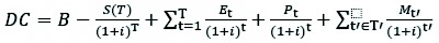
During the life of the equipment, the operating costs usually increase, equipment availability decreases, and salvage value declines, reflecting the remaining contribution of the equipment to the enterprise or to others (Diniz and Sessions 2020). In such an environment, the discounted cost over the equipment life, considering a specific planning horizon (Bowman and Fetter 1967) for the discrete case is:

(1)

Where:

DC discounted cost

B purchase price of the new equipment at time 0

S(T) salvage value of the equipment of age T

E operating and maintenance cost at time t

P cost at time t for the lost production at time t

Mt’ overhaul cost at time t’ where t’ is in the set T’ of overhaul times. The overhaul components are tires, tracks, hydraulic pump, harvester head and engine

I discount rate.

We propose a solution method called EPSDS. A Microsoft Excel workbook containing ESPDS may be found on the web at the following URL: https://www.researchgate.net/publication/350811380_ESPDS_workbook. The workbook is organized into four worksheets. The first worksheet shows how to use ESPDS in six steps. The input data is entered in the second and third spreadsheets (e. g., purchase price, discount rate, planning horizon). The fourth worksheet shows the decision-maker which equipment better suits their operation. The problem formulation is described by the logic diagram in Fig. 1.

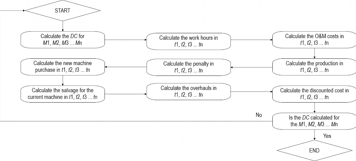
Fig. 1 Logic diagram to calculate discounted cost (DC) by Eq. 1

2.2 How Does ESPDS Work?

ESPDS can be applied to support companies and contractors to choose the best equipment option for their operations, as well as to achieve better equipment purchase agreements. ESPDS can also be useful for providing longer term estimates of production costs. Through a sensitivity analysis, it is possible to test different maintenance polices and new technologies.

The procedure begins with the identification of the planning horizon and the equipment to be considered. As mentioned earlier, we are assuming that the decision-maker has already selected all equipment options for purchase. The next step is to add the input data to the program. ESPDS requires specific cost-related inputs, such as equipment purchase price, residual value, discount rate, maintenance policies, penalty for unproductive hours, work schedule, operation and maintenance (O&M) costs, utilization rate, and productivity.

ESPDS has 6 steps.

Step 1. Identify the desired machines to apply the equipment selection algorithm.

Step 2. Define the planning horizon (years), and the discount rate to be used in the process. The discount rate is the expected rate of return that is used to adjust cash flows for the time value of money.

Step 3. Enter the values as the purchase price, residual value, schedule, and an optional production penalty. A production penalty is applied if the availability of the equipment falls below a specified level, and a substitute machine must be »rented« to make up the lost production. Thus, during the hours of non-operation, the work is done by a contractor, so that the company’s production target can be met.

Step 4. Enter with utilization rate, O&M costs, productivity and the scheduled hours of operation over the machine life.

Step 5. Indicate the maintenance policy for all equipment considered. The maintenance policy specifies cost and timing of components such as tires, tracks, hydraulic pump, engine, and implement (e.g., head and grapple).

Step 6. Run the algorithm for all equipment considered. The best solution is the lowest discounted production cost over the planning horizon.

2.2.1 Input Data

The ESPDS workbook consists of an introduction section; input section (Fig. 2) where cost and equipment data are entered; and an output section (Fig. 3) where the results are presented. The main input section is divided into four parts. First, the decision-maker needs to enter data such as schedule (h/y), annual discount rate (%), purchase price ($), residual value (%), penalty ($/h), and planning horizon (y).

In the second part, the decision-maker needs to add overhaul information, such as the expenses to replace the items and the time over the planning horizon. For example, we need to replace tires with 8000 hours and, to do that, it will cost around $13,000. In the third part, the decision-maker will add the maintenance policy over the equipment life. Depending on the replacement time for each item, it is possible that some replacements will cost more than others. Using the previous example, the first major replacement would be at 8000 hours. In this way, the next tire replacement would be at 16,000 hours, and so on.

The last and the most challenging part is where the decision-maker needs to add specific data on productivity, utilization rate, and O&M costs. As we mentioned earlier, during the life of the equipment, operating costs generally increase and the availability of the equipment decreases, as does its productive capacity. In the case of productivity, we believe that productive capacity will decrease as the implement ages.

In order to calculate the O&M costs, productivity, and utilization, the company’s historical database was used, making it possible to obtain reliable values that fit the scope of the decision. We chose not to use continuous equations to estimate O&M costs, as they occur less frequently, and can affect the replacement decision. To calculate the productivity of the equipment for each month, we used a constant tree size. This could also have been varied over the planning horizon if suggested by the strategic plan.

In the first column, as shown in Fig. 2, the decision-maker inserts the operational hours over the equipment life. In the second and third columns, the utilization rate and O&M costs data are added, according to the equipment lifetime. In the fourth column, the values of productivity are added. In the Appendices, it is possible to access the database used for each equipment. Therefore, the decision maker can have an idea of how the data can be inserted into the input worksheet. As Ackerman et al. (2014) noted, the precision of the output will be a reflection of the accuracy of the data input.

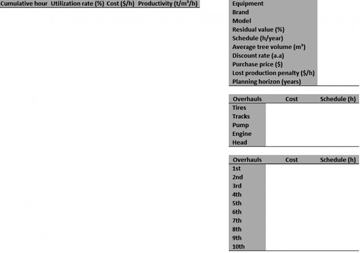
Fig. 2 The input section of the spreadsheet

2.2.2 Outputs

In the output section, the results are presented by three main variables: accumulated discounted cost, accumulated production, and production cost over the desired planning horizon. As Fig. 3 shows, it is also possible to check the production cost over the life of the equipment, as well as the evolution of the operating cost. After running the cash flow calculations, ESPDS shows which equipment has the lowest production cost, helping the decision-maker to identify the best equipment for its operation. It provides a comprehensive breakdown of all costs in monetary terms. Equipment operating costs over longer planning horizons can be estimated so that longer-term capital investments can have projected costs that are consistent with longer-term projections.

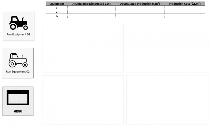
Fig. 3 The output section of the spreadsheet

2.3 Numerical Example

To demonstrate ESPDS, we illustrate the equipment selection problem using five tree harvesting machines of a large integrated Brazilian forestry company in southern Brazil. Table 1 provides the input data including schedule, discount rate, purchase price, residual value, penalty, planning horizon, and overhaul costs. As in Diniz and Sessions (2020), items such as utilization rate, O&M costs and productivity vary over the useful life of the equipment rather than assuming average values which could leave the best alternative far from reality. The detailed input data (utilization rate, O&M costs, and productivity) are available in the appendix section.

Table 1 List of data used

It is important to highlight that three of the equipment were of the same brand and model, and had the same purchase price (see Table 1). In order to test different scenarios, we use different maintenance policies, varying not only the exchange time for each item but also the type of part – e.g. tires, hydraulic pump, and engine. This explains the different costs of equipment overhaul, as well as the different maintenance schedules. Table 2 presents the different maintenance policies for each equipment considered.

Table 2 Maintenance policies for each equipment

According to Ackerman et al. (2014), when a dealer’s asking price for used equipment includes the dealer’s profit, the asking price will usually be considerably higher than the salvage value the dealer pays when the dealer buys the machine. In this sense, we are taking into account a straight line method to calculate the residual value over the desired planning horizon. This assumes that the value of equipment decreases at a constant rate of its economic life. We also used the same production penalty applied in Diniz and Sessions (2020) to make up the lost production during the hours of non-operation. The work could be done by a contractor, so that the company’s production target can be met.

3. Results

3.1 Numerical Results

Fig. 4 shows the accumulated discounted costs for equipment over the planning horizon. We observed that all equipment had similar discounted costs, although Equipment 5 has the highest discounted costs. Factors that explain the higher discounted cost presented by Equipment 5 are the purchase price and O&M costs - see Table 1 and the appendix section.

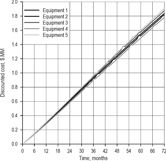
Fig. 4 Cumulative discounted cost for each equipment over the planning horizon

From Fig. 5, the production cost generally increases over the planning horizon, due to increases in the O&M costs and decreases in utilization rate, making the penalty paid for unproductive times ever higher. After the 40th month of the planning horizon, production costs fall slightly, reflecting the replacement of the harvesting heads, which allow for productivity gains.

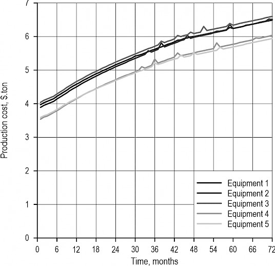
Fig. 5 Production cost for each equipment over the planning horizon

According to Table 3, Equipment 5 presented the lowest production cost, indicating it was the best alternative to purchase so far. Nevertheless, assume that the decision maker does not have the total funds necessary to purchase Equipment 5. He could try to negotiate with the dealer to obtain a discount on the purchase price, however, if he was not successful, he could choose to purchase Equipment 4, which showed little variation from Equipment 5 in the cost of production and requires a lower initial investment.

Table 3 Results presented for each equipment after running the equipment selection tool

Another option would be to invest in a new technology, which would make it possible to increase productivity or increase the utilization rate. Section 3.3 presents the simulation of an example, considering the entrance of a new technology that allows an increase in the productivity of 2%.

3.2 Sensitivity Analysis

To verify which input data had the greatest influence on the production cost, we increased and decreased the initial purchase price, penalty, discount rate, O&M costs, utilization, productivity, and overhauls by 2.5% and 5% for Equipment 5 with all other inputs held constant. Fig. 6 shows the impact of those changes on the production cost.

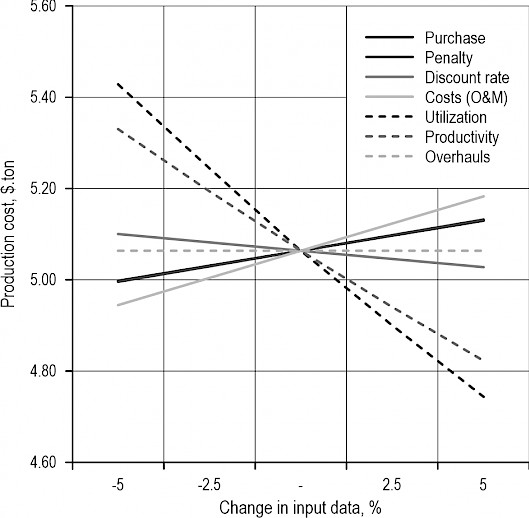
Fig. 6 Production cost of Equipment 5 considering an increase and decrease of 2.5% and 5% in the input data

3.3 Entrance of New Technology

In addition to showing the versatility of ESPDS in simulating future scenarios that can help decision makers to identify the best equipment for their operation, we introduce a case of new technology, which is already being tested with forestry equipment and will be the subject of our next work. Changes to electronic injection by reprogramming the engine control unit (ECU) (e.g., Hafner and Isermann 2003, Sequenz and Isermann 2011) create different engine performance characteristics, depending on the company's or contractor's objective.

For example, if the machine owner has equipment that is unable to perform its job satisfactorily due to lack of power or torque, it is possible, through fine adjustments in the original ECU map, to obtain more power and torque. If the goal is to reduce the fuel consumption of the equipment, it is possible to modify the torque curve so that the engine operates in a lower rpm range, reducing fuel consumption. For ESPDS testing purposes, we simulated an adjustment to the ECU map that increased the productivity of Equipment 4 by 2%, keeping all other variables as they were. We also added a $2000 investment needed to obtain this new optimized map. Figs. 7, 8 and Table 4 show the results obtained after performing ESPDS for Equipment 4 and 5.

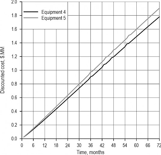
Fig. 7 Cumulative discounted cost for each equipment over the planning horizon considering the entrance of a new technology

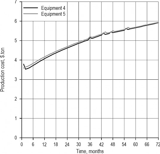
Fig. 8 Production cost for each equipment over the planning horizon considering the entrance of a new technology

Table 4 Results presented by Equipment 4 and 5 after running the equipment selection tool considering the entrance of a new technology

4. Discussion

4.1 Numerical Results

O&M costs can be a difficult task to predict because they can change according to operating conditions, operator skills, and maintenance policies (Brinker et al. 2002, Dodson et al. 2015, Di Fulvio et al. 2017, Diniz et al. 2020a). As mentioned earlier, in order to apply ESPDS, it is necessary to obtain these cost curves.

Ackerman et al. (2014) adopted a different strategy from our approach. They represented maintenance costs in an aggregated way and were not specific in details. Although this permits users without good long-term records to use their model, it may provide misleading results. For this reason, we emphasize the importance of using precise input data (O&M costs, utilization rate, and productivity over the equipment life).

When it is not possible to access quality information, reliability decreases. When it is possible to access good quality information, detailed models end up working very well, as observed by Ackerman et al. (2014). Also, from Fig. 5, the decision maker can see the impact of the maintenance policies on the cost of production. When there is a need for a major overhaul, production costs increased considerably. However, it is a necessary expense, otherwise, production costs could increase even more due to equipment failures and lost productivity.

At this point, the decision maker is able to identify the best equipment for his operation. The line closest to the horizontal axis represents the best choice. Even with the highest discounted costs – see Fig. 4, Equipment 5 proved to be superior to the others (see Table 3). This result is explained by a higher utilization rate and higher productivity. It is clear that to achieve this result, there was a combination of other variables (e.g., purchase price, O&M costs, discount rate), which were at a level that made such a result possible. Equipment 4 showed similar results, which despite having a higher production cost, requires fewer resources than Equipment 5.

Another benefit of applying ESPDS is to obtain detailed cost schedules – see Fig. 5. Forest harvest scheduling decisions often require estimates of future harvest costs. These projections of future conditions directly provide a consistent link between the decision to purchase one or more pieces of equipment and the strategic plan of the company or contractor (Diniz and Sessions 2020).

4.2 Sensitivity Analysis

Sensitivity analyses using ESPDS is recommended to test how the result changes if inputs are changed. This process is important, especially for cost items that make up a relatively large share of the total costs, such as purchase price, O&M costs, utilization rate and productivity, or where the input data are of a lower quality.

We look at the results in Fig. 6 from three perspectives: (1) the variables that most affect the production cost: utilization rate and productivity, (2) the variables that affect the production cost with less intensity: O&M costs, purchase price, and penalty and (3) the variables that have little influence on the cost of production – discount rate and overhauls.

Of the three groups, the first one is the most important. This information can lead the decision maker to make better purchasing agreements, as well as to seek better maintenance practices and test new technologies (next section) to reduce production cost. Diniz et al. (2020b) show in their work that better maintenance practices lead to increases in the forestry equipment utilization rate.

Knowing that the purchase price has less influence on the production cost than utilization rate, it is possible to negotiate with the dealer some type of agreement in which he undertakes to maintain a minimum utilization rate in the first year, guaranteeing a degree of stability to the contractor.

Although the purchase price had less impact than the utilization rate and productivity, it is necessary to keep attention on this variable. According to Ackerman et al. (2014), the stated purchase price for a machine will often differ by more than 10% depending on whether the retailer or the contractor is asked. The dealer usually gives a price for a minimum configuration of the machine. At this point, the decision-maker needs to consider doing sensitivity analysis to make sure the best alternative is near to reality.

Another important point that can be drawn from this analysis is that this information provides guidance for many researchers working with forestry operations. For example, in our analysis it has been shown that the utilization rate and productivity are the factors that have the greatest influence on production cost. This can direct future work to test new technologies, as well as maintenance practices that have not yet reached forestry operations.

4.3 Entrance of New Technology

To increase the productivity of the equipment, Spinelli and Moura (2019) tested an adaptation kit, specifically designed to improve communication between the harvester head and the excavator. According to the authors, there was a 6% increase in equipment productivity. However, the kit presented in their study was not developed for universal use. An example of a new technology that can be applied to any type of equipment is the use of new grid maps on the electronic central unit (ECU), which allow equipment to increase power and productivity.

We assume no negative engine effects from this new map and we may need to study them in practice. It is possible that, when using an inappropriate map, peripherals such as the turbocharger turbine may have a shorter life, reducing the equipment utilization rate. Fig. 7 showed the results obtained after performing ESPDS for Equipment 4 and 5. As can be seen, Equipment 5 still has higher discounted cost, however, it is still necessary to verify how much each equipment will produce over the planning horizon.

We also found that, unlike Fig. 5, the production cost of Equipment 4 fell slightly. During the second month, Equipment 4 had an increase in its production cost, which was due to the investment decision to buy and install the new ECU map. It is possible to verify that increasing the productivity of Equipment 4 by 2% is sufficient to reduce its production cost and Equipment 4 now becomes an attractive option for decision-makers. Using the sensitivity analysis, it was already possible to identify that investing in a technology that provides productivity gains would have a positive effect.

Table 4 shows that Equipment 4 increased its production over the planning horizon and the amount invested in the new electronic injection map had negligible impact on the discounted cost. The cost of production fell by $ 0.02. At this point, ESPDS helped the decision-maker to identify that the best equipment for his activity would be Equipment 4.

Our hope is that, through ESPDS, contractors, companies, and researchers can make the selection of equipment simply, quickly and that the results portray a possible reality. The limiting restriction on its use is to carefully identify the input data. As Ackerman et al. (2014) identified, the use of estimates and erroneous data can lead to poor quality analyses.

5. Conclusions

We have described a Workbook containing ESPDS for the selection equipment problem. The ESPDS simulator can calculate the accumulated production and the discounted cost of logging operations over the desired planning horizon, as well as the production cost, assisting contractors in selecting the equipment that best suits their operation. The numerical example showed us the Equipment 5 was the better option to buy. Although Equipment 5 presented higher accumulated discounted costs, its productivity proved to be enough to get lower production costs. When we explored the sensitivity of the solution to varying input assumptions and rerunning ESPDS, the impacts of those variations show the most influencing factor on the production cost was the utilization rate, illustrating that improvements in maintenance techniques could provide benefits to the contractor. When considering the entrance of new technology, ESPDS showed the best alternative shifted to Equipment 4 as a result of the productivity gain from modifying the ECU map. While the results of reprogramming the ECU have been obtained through simulation, we are currently exploring this new technology in a real case with promising results. We have illustrated the use of ESPS with a harvester, but ESPDS has the potential to support the planning of short- to long-term logging management with other equipment and can be easily adapted to other sectors.

6. References

Ackerman, P., Belbo, H., Eliasson, L., de Jong, A., Lazdins, A., Lyons, J., 2014: The COST model for calculation of forest operations costs. International Journal of Forest Engineering 25(1): 75–81. https://doi.org/10.1080/14942119.2014.903711

Amini, S., Asoodar, M.A., 2016: Selecting the most appropriate tractor using analytic hierarchy process – An Iranian case study. Information Processing in Agriculture 3(4): 223–234. https://doi.org/10.1016/j.inpa.2016.08.003

Bilek, E.M., 2007: ChargeOut! Determining machine and capital equipment charge-out rates using discontinued cash-flow analysis. U.S. Department of Agriculture, Forest Service, Forest Products Laboratory, General technical report Nr. FPL-GTR–171.

Bowman, H., Fetter, R.B., 1967: Analysis for production and operations management. 3rd ed. Homewood (IL): Richard D. Irwin, Inc.

Brinker, R.W., Kinard, J., Rummer, B., Lanford, B., 2002: Machine rates for selected forest harvesting machines. Auburn (AL): Alabama Experiment Station, 32 p.

Brunberg, T., 1997: Basic data for productivity norms for single-grip harvesters in thinning. Skogsforsk Redogörelse 8: 18.

Cantú, R.P., LeBel, L., Gautam, S., 2017: A context specific machine replacement model: a case study of forest harvesting equipment. International Journal of Forest Engineering 28(3): 124–133. https://doi.org/10.1080/14942119.2017.1357416

Chiorescu, S., Grönlund, A., 2001: Assessing the role of the harvester within the forestry-wood chain. Forest Products Journal 51(2): 77–84.

Çimren, E., Çatay, B., Budak, E., 2007: Development of a machine tool selection system using AHP. The International Journal of Advanced Manufacturing Technology 35(3–4): 363–376. https://doi.org/10.1007/s00170-006-0714-0

Di Fulvio, F., Abbas, D., Spinelli, R., Acuna, M., Ackerman, P., Lindroos, O., 2017: Benchmarking technical and cost factors in forest felling and processing operations in different global regions during the period 2013–2014. International Journal of Forest Engineering 28(2): 94–105. https://doi.org/10.1080/14942119.2017.1311559

Diniz, C., Sessions, J., 2020: Ensuring consistency between strategic plans and equipment replacement decisions. International Journal of Forest Engineering 31(3): 211–223. https://doi.org/10.1080/14942119.2020.1768769

Diniz, C., Sessions, J., Junior, R.T., Robert, R., 2020a: Equipment replacement policy for forest machines in Brazil. International Journal of Forest Engineering 31(2): 87–94. https://doi.org/10.1080/14942119.2020.1695514

Diniz, C., Lopes, E.S., Koehler, H.S., Miranda, G.M., Paccola, J., 2020b: Comparative analysis of maintenance models in forest machines. Floresta e Ambiente 27(2): 1–7. https://doi.org/10.1590/2179-8087.099417

Dodson, E., Hayes, S., Meek, J., Keyes, C.R., 2015: Montana logging machine rates. International Journal of Forest Engineering 26(2): 85–95. https://doi.org/10.1080/14942119.2015.1069497

FAO, 1992: Cost Control in Forest Harvesting and Road Construction. FAO, Rome. Forestry papers Nr. 99, 16 p.

Gellerstedt, S., Dahlin, B., 1999: Cut-to-length: the next decade. Journal of Forest Engineering 10(2): 17–25.

Hafner, M., Isermann, R., 2003: Multiobjective optimization of feedforward control maps in engine management systems towards low consumption and low emissions. Transactions of the Institute of Measurement and Control 25(1): 57–74. https://doi.org/10.1191/0142331203tm074oa

Hogg, G., Längin, D., Ackerman, P., 2010: South African Harvesting and transport costing model. Department of Forest and Wood Science, Stellenbosch University, 37 p.

Karim, R., Karmaker, C.L., 2016: Machine selection by AHP and TOPSIS methods. American Journal of Industrial Engineering 4(1): 7–13. https://doi.org/10.12691/ajie-4-1-2

IBA - Brazilian Tree Industry, 2019: Annual report 2019. https://iba.org/datafiles/publicacoes/relatorios/iba-relatorioanual2019.pdf.

Lundbäck, M., Häggström, C., Nordfjell, T., 2018: Worldwide trends in the methods and systems for harvesting, extraction and transportation of roundwood. In: International Forest Engineering Conference, 6, Rotorua: SOBAMA, 1–3.

Matthews, D.M., 1942: Cost control in the logging industry. New York: McGraw-Hill book company, 374 p.

Miyata, E.S., 1980: Determining fixed and operating costs of logging equipment. General Technical Report NC-55. Forest Service North Central Forest Experiment Station, St. Paul, MN, 14 p.

Nurminen, T., Korpunen, H., Uusitalo, J., 2006: Time consumption analysis of the mechanized cut-to-length harvesting system. Silva Fennica 40(2): 335–341. https://doi.org/10.14214/sf.346

Nguyen, T.P.K., Yeung, T.G., Castanier, B., 2013: Optimal maintenance and replacement decisions under technological change with consideration of spare parts inventories. International Journal of Production Economics 143(2): 472–477. https://doi.org/10.1016/j.ijpe.2012.12.003

Sequenz, H., Isermann, R., 2011: Emission model structures for an implementation on engine control units. Proceedings of the 18th World Congress. The International Federation of Automatic Control, Milano (Italy) August 28 – September 2.

Spinelli, R., Magagnotti, N., Picchi, G., 2011: Annual use, economic life and residual value of cut-to-length harvesting machines. Journal of Forest Economics 17(4): 378–387. http://dx.doi.org/10.1016/j.jfe.2011.03.003

Spinelli, R., Moura, A.C.A., 2019: Decreasing the fuel consumption and CO2 emissions of excavator-based harvesters with a machine control system. Forests 10(43): 1–12. https://doi.org/10.3390/f10010043

Sundberg, U., Silversides, C.R., 1988: Operational efficiency in forestry. Doordrecht, the Netherlands, Kluwer academic publishers, 219 p.

Yurdakul, M., 2004: AHP as a strategic decision-making tool to justify machine tool selection. Journal of Materials Processing Technology 146(3): 365–376. https://doi.org/10.1016/j.jmatprotec.2003.11.026

© 2021 by the authors. Submitted for possible open access publication under the
terms and conditions of the Creative Commons Attribution (CC BY) license (http://creativecommons.org/licenses/by/4.0/).

Authors’ addresses:

Carlos Diniz, PhD *

e-mail: carloscezardiniz@gmail.com

Federal University of Parana

632, Lothário Meissner Avenue

Curitiba PR 80210-170

BRASIL

Prof. John Sessions, PhD

e-mail: john.sessions@oregonstate.edu

Oregon State University

College of Forestry

336 Peavy Forest Science Complex

Corvallis OR 97331-5704

USA

* Corresponding author

Received: September 03, 2020

Accepted: September 13, 2021

Original scientific paper