Introducing a New Approach in Stand Tending Planning and Thinning Block Designation by Using Mixed Integer Goal Programming

Long-term management plans have been developed for nearly all of the forests in Turkey. These plans are applied at a sub-district management unit level and may contain guidance for both intermediate yield and final yield harvests. To implement an intermediate yield plan, which involves the scheduling of forest thinnings (stand tending), consideration in Turkey is given to the advantages of working in the same terrain and the same general area each year. Therefore, compartments are often clumped together to create thinning blocks, taking into consideration the thinning priority of the stands, road conditions, site index, age, and proximity of the compartments. Further, when preparing annual budgets and planning to meet the market’s needs, forest enterprises require an even flow of intermediate wood volume each year. In this paper, we introduce a new approach in stand tending planning designed to schedule an equal amount of intermediate wood volume each year and to create thinning blocks by minimizing the distance to pre-defined ramps (landings). We developed both linear and nonlinear goal programming models to minimize both the deviations from a harvest volume (annual intermediate yield allowable cut) target and the deviations from a target value determined for the distances (total and average) of the centroid of each compartment to the hypothetical forest ramps. By using the extended version of Lingo 16, we solved the problem with different weights for the deviations in volume and distance that ranged from 0.0 to 1.0, in 10% intervals, which created 11 scenarios. We carefully analyzed the results of each scenario by taking into consideration the wood volume and distance of compartments to the ramps. The best scenario using the linear model produced a deviation in volume scheduled for the entire decade of 6 m3, while the deviation in total distance between harvest areas and ramps was 59.7 km. Scenario 5, with weights of 0.6 for volume and 0.4 for distance, produced these results, where compartments were closest to one another. The best scenario using the nonlinear model also produced a deviation in volume of 0 m3 and the total average deviation in distance between harvest areas and ramps was 8.7 km. Scenario 3, with weights of 0.8 for volume and 0.2 for distance, produced these results. The approach and models described through this study may be appropriate for further integration into forest management planning processes developed for the planning of Mediterranean forests.

Introducing a New Approach in Stand Tending Planning and Thinning Block Designation by Using Mixed Integer Goal Programming

Mehmet Demirci, Ahmet Yesil, Pete Bettinger

Abstract

Long-term management plans have been developed for nearly all of the forests in Turkey. These plans are applied at a sub-district management unit level and may contain guidance for both intermediate yield and final yield harvests. To implement an intermediate yield plan, which involves the scheduling of forest thinnings (stand tending), consideration in Turkey is given to the advantages of working in the same terrain and the same general area each year. Therefore, compartments are often clumped together to create thinning blocks, taking into consideration the thinning priority of the stands, road conditions, site index, age, and proximity of the compartments. Further, when preparing annual budgets and planning to meet the market’s needs, forest enterprises require an even flow of intermediate wood volume each year. In this paper, we introduce a new approach in stand tending planning designed to schedule an equal amount of intermediate wood volume each year and to create thinning blocks by minimizing the distance to pre-defined ramps (landings). We developed both linear and nonlinear goal programming models to minimize both the deviations from a harvest volume (annual intermediate yield allowable cut) target and the deviations from a target value determined for the distances (total and average) of the centroid of each compartment to the hypothetical forest ramps. By using the extended version of Lingo 16, we solved the problem with different weights for the deviations in volume and distance that ranged from 0.0 to 1.0, in 10% intervals, which created 11 scenarios. We carefully analyzed the results of each scenario by taking into consideration the wood volume and distance of compartments to the ramps. The best scenario using the linear model produced a deviation in volume scheduled for the entire decade of 6 m3, while the deviation in total distance between harvest areas and ramps was 59.7 km. Scenario 5, with weights of 0.6 for volume and 0.4 for distance, produced these results, where compartments were closest to one another. The best scenario using the nonlinear model also produced a deviation in volume of 0 m3 and the total average deviation in distance between harvest areas and ramps was 8.7 km. Scenario 3, with weights of 0.8 for volume and 0.2 for distance, produced these results. The approach and models described through this study may be appropriate for further integration into forest management planning processes developed for the planning of Mediterranean forests.

Keywords: linear goal programming, nonlinear programming, mixed integer goal programming, optimization, thinning schedule intermediate yield planning

1. Introduction

Forests, as major components of terrestrial ecosystems, provide to society many economic, environmental and socio cultural services. Forests provide favourable mid-term green growth opportunities, they also facilitate the attainment of long-term ecosystem services that include the mitigation of climate change and the production of clean air and water (United Nations Food and Agriculture Organization 2016). In order to ensure these services are available in the long-run, the use of sustainable forest management principles becomes more important. Forest management plans can be developed to illustrate how the outcomes that represent measurable achievement of these services can be obtained through management activities. While a forest management plan has been developed for nearly all of the forests in Turkey, long-term forest management plans have been developed for only about 54% of the world’s forests (United Nations Food and Agriculture Organization 2020).

In Turkey, forest management plans are developed for sub-district management units, and they can provide guidance for both final (regeneration harvest) and intermediate (thinning/stand tending) management activities. One of the main considerations for intermediate harvest activities is that they are placed in close proximity during each year of a management plan, so that workers conduct activities in similar terrain and in the same general area. In this sense, compartments (collections of stands) are combined to create operational thinning blocks. In addition, the thinning blocks do not include stands that have a final harvest scheduled, during the first period (10 years). The scheduled thinning activities take into consideration the silvicultural need for thinning stands, marketing opportunities, and road system conditions. Finally, the yield from intermediate harvests would ideally be consistent from year to year to facilitate the market’s needs (Eraslan 1982).

In conducting this research, the harvest scheduling aspects related to wood flow and location of intermediate harvest management activities were recognized. The total and average distances of the scheduled intermediate harvest compartments to the forest ramps (areas where logs are loaded for transport to a woodyard or mill) were also included. The forest ramps were hypothetical and located throughout the planning unit. They are typically developed when they are needed, thus they were randomly located, yet checked for plausibility by the lead author based on his expertise as a forest engineer and his familiarity with the landscape. The total distance of the compartments to the ramps was used for the linear model, and the average distance, which was obtained by dividing the total distance by the number of scheduled compartments, was used for the non-linear model. From the suite of operations research techniques that have been used in management planning, goal programming (GP) is suitable for addressing this type of complex forestry problem that has more than one consideration in the objective function (Demirci and Bettinger 2015). And since we assume that entire compartments will be scheduled for intermediate harvests, a mixed integer approach is needed to ensure that activities within compartments are fully scheduled within a single year. In accommodating the distance to ramps, goal problem formulations were designed using both linear GP and nonlinear GP.

GP has been widely used in many different fields of commerce. The process was initially described by Charnes et al. (1955) as an alternative use of linear programming. The term »goal programming« was attributed to this process by Charnes and Cooper (1961). Rustagi (1973) and Field (1973) provide the first demonstrations of GP in forest management. A number of other works have demonstrated how GP can be applied to traditional forest management objectives that have commodity production, economic, and other objectives (Porterfield 1973, 1974, Lyon 1974, Romesburg 1974, Bell 1975, Dress 1975, Schuler and Meadows 1975, Bare and Anholt 1976, Schuler et al. 1977, Kahalas and Groves 1978, Kao and Brodie 1979, Field et al. 1980, Köse 1986, Kangas and Pukkala 1992, Diaz-Balteiro and Romero 1998, Misir 2001, Bertomeu and Romero 2001, 2002, Diaz-Balteiro and Romero 2003, Misir and Misir 2007, Silva et al. 2010, Gómez et al. 2011, Chen et al. 2011, Aldea et al. 2014, Chen and Chang 2014, Zengin et al. 2015). The features within an objective function of a GP problem can be weighted using several approaches and schemes to emphasize the importance of objective function components or to normalize the values of disparate outcomes such as wood flow and wildlife habitat (Hotvedt et al. 1982, Hotvedt 1983, Hossain and Robak 2010). The spatial location of harvest activities has also been recognized in GP problems to control the timing and placement of management activities (Demirci and Bettinger 2015, Augustynczik et al. 2016, Bagdon et al. 2016).

The aim of this study is to develop two mixed integer GP models that address the intermediate harvest activities typical of the Turkish forest management problem in a different manner for each period in this area (e.g., Demirci and Bettinger 2015). A linear thinning model (LTM) and a nonlinear thinning model (NLTM) were developed to minimize deviations from the wood flow target and the distance to the forest ramp (total and average) target. To be clear, the problem-solving method involves mixed integer GP, although a portion of the problem formulation involves either linear or nonlinear functions to represent the spatial constraints.

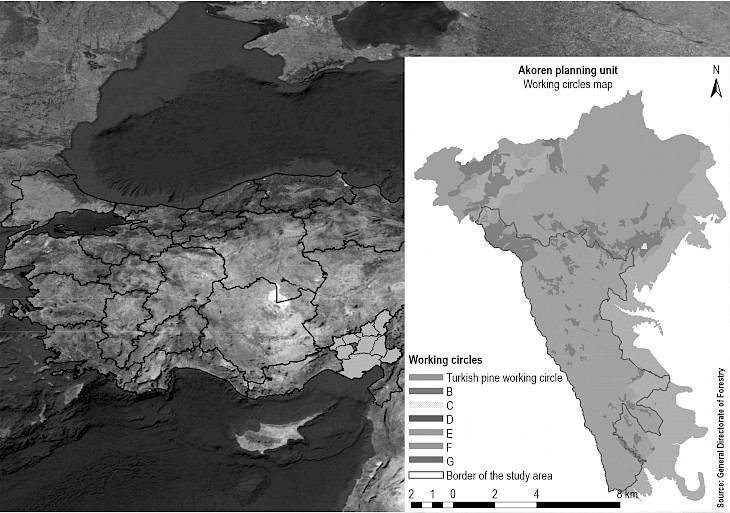
Fig. 1 Location of Akoren Planning Unit and study area (Turkish pine working circle)

2. Materials and Methods

2.1 Case Study

Located in the Mediterranean region of Turkey (Fig. 1), the study area is a sub-set of the Akoren Planning Unit of the Adana Forest Regional Directorate. The study area contains about 5380 ha of coniferous forests. Turkish pine (Pinus brutia Ten.) is the dominant coniferous tree species, and other coniferous species include Anatolian black pine (Pinus nigra Arn. subsp. pallasiana (Lamb.) Holmboe var. pallasiana), fir (Abies cilicica Carr.), cedar (Cedrus libani A. Rich.), and juniper (Juniperus spp.). The estimated growing stock of the study area is 559,006 m3 and the annual increment of the growing stock is 22,422 m3 (increment of thinning stands is 8324 m3). The production of pine wood volume is the main management objective of the study area. Plans are developed for the study area every 20 years, and the length of the thinning cycle is 10 years.

Thinning operations during the first decade are conducted within compartments that do not have other stands scheduled for a final harvest during that decade. For comparison and use in this analysis, the area, increment, growing stock, and allowable cut information for the planned thinning compartments were obtained from the Forest Plan of the Akoren Planning Unit (General Directorate of Forestry 2014). This information was developed using spreadsheet-based analysis of forest information. The number of thinning compartments in the study area is 84, and the estimated annual allowable cut for these compartments is 2628 m3 per year (about 32% of the 8324 m3 increment of thinning stands) (Table 1).

Table 1 Stand tending compartments and their annual allowable cuts

In this research, the objective was to schedule for harvest a set of thinning compartments in such a way that they were physically close to each other each year. This arrangement would in effect ease the work organization for the foresters and reduce losses in labour time, and cost for moving machinery and equipment. For this work, 10 hypothetical forest ramps (landings) were located throughout the study area (Fig. 2). Using the Calculate Geometry tool within ArcMap, the latitude and longitude positions of the ramps and the centroid of each compartment were determined. The Euclidian distance from each ramp to each compartment was then calculated. In sum, 840 ramp-compartment distance combinations were produced between the 84 compartments and 10 ramps.

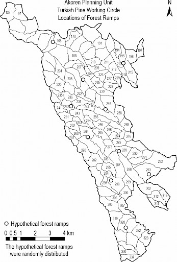
Fig. 2 Locations of hypothetical forest ramps

2.2 Problem Formulation

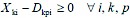
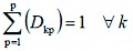
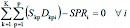
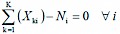
To address the scheduling of thinnings throughout the study area, it is desired to minimize both the deviations from a desired harvest volume (annual intermediate yield allowable cut) and the distances (total and average) from each compartment to a ramp over a 10-year time horizon. The foresters also want to thin the forests within each compartment as a whole when they are entered; therefore, the decision for a compartment is discrete (to harvest or not to harvest). Given this management situation, mixed integer GP may be useful in scheduling the thinning activities.We designed both a mixed-integer linear GP model and a mixed-integer nonlinear GP model to address this thinning problem. The mathematical formulation of the mixed-integer linear thinning GP model (LTM) is as follows:

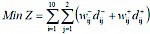(1)

Subject to

(2)

(3)

(4)

(5)

(6)

(7)

(8)

(9)

(10)

(11)

(12)

(13)

Where:

i years

j objectives: 1 = volume scheduled for harvest, 2 = distance of compartments to a forest ramp

weight for negative deviations in objective j, year i

weight for positive deviations in objective j, year i

negative deviation in objective j, year i

positive deviation in objective j, year i

K total number of compartments within the planning unit

k a compartment within the planning unit

binary (0, 1) decision variable representing the harvest of compartment k during year i

volume available for harvest in compartment k during year i

total volume scheduled for harvest in year i

P total number of forest ramps

p a forest ramp

a binary (0,1) variable representing the distance of compartment k to forest ramp p, in year i

distance between the centroid of compartment k and forest ramp p

total distance of the centroids of scheduled compartments in year i

number of scheduled compartments in year i

volume target in year i

distance target in year i.

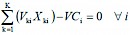
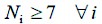
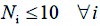
Eq. 1 represents the objective function, which minimizes the deviations from volume and distance targets. The harvest target for Eq. 11 was 2628 m3, and the distance target for Eq. 10 was assumed to be 7 km. Eq. 2, together with Eq. 12, forces a compartment to be scheduled for harvest. Eq. 3 represents the accounting rows that sum harvest volumes each year. Eq. 4 determines the pairs of compartments and forest ramps in the same year. Eq. 5, together with Eq. 13, forces only one »scheduled compartment-forest ramp« pair to be considered in the same year. Eq. 6 represents the accounting rows that sum the distances between scheduled compartments and forest ramps. Eq. 7 counts the compartments scheduled for harvest for each year. Eqs. 8 and 9 limit the number of compartments scheduled for harvest for each year, since foresters want to manage roughly the same number of compartments each year. Since it was not possible to equalize the numbers of the compartments scheduled for harvest each year, Eqs. 8 and 9 were used to limit the maximum and minimum number of the compartments scheduled for harvest. These levels (minimum 7 and maximum 10) were determined based on the results of previous (trial) model runs. Eq. 10 calculates the deviations in volume scheduled for harvest from the volume target. Eq. 11 calculates the deviations in distances of scheduled compartments to ramps from the distance target.

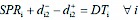
The mathematical formulation of the mixed-integer nonlinear GP model (NLTM) is similar to the LTM model with a few exceptions. To make the above linear mathematical formulation nonlinear, we added the following equation:

(14)

Where:

AVDi the average distance between scheduled compartments for harvest and forest ramps in year i.

In this nonlinear case, in Eq. 11, AVDi replaces SPRi and DTi represents the desired average distance between scheduled compartments for harvest and forest ramps. In this case, the deviation from the average distance replaces the total distance in the objective function. Here, we assumed a 1 km target for the distances between harvest units in a year. In effect, these changes attempt to clump thinning harvests together regardless of their distance to a ramp.

LINGO 16.0 (Lindo Systems, Inc. 2016) was used to solve these problems, where an unlimited number of continuous value, integer, and nonlinear variables were accommodated. Some data was exported from a geographic information system (GIS) to text files to address the need for distances amongst landscape features, and Lingo syntax was developed in a spreadsheet and text editor. The total number of variables and constraints within these models was moderately large (Table 2). The problems further used different weights in the objective function to represent the importance of deviations in harvest volume and compartment distance. The weights ranged from 0.0 to 1.0, in 10 percent intervals, and thus 11 scenarios were created for each of the two models (Table 3). Weights were applied to the objective function variables in order to observe how sensitive changes in volume and distance outcomes were when the emphasis between these two was altered. Either method (weighting or normalizing) can be used to reduce unintentional bias towards the parts of the objective that have a larger magnitude, and weighting has been put forward as one way to normalize outcomes (Tamiz et al. 1998, Kettani et al. 2004). A PC with a 2.60 GHz Intel® Core™ i7 processor and 16 GB of RAM was used to run LINGO. If the optimum solution was not located prior to about 100 million iterations of the LINGO model, the best solution located during the branch and bound search was reported (Table 4).

Table 2 Total number of variables and constraints used in two models (LTM and NLTM)

Table 3 Weights for two objectives

Table 4 Total solver iterations and elapsed runtime seconds for linear and nonlinear models

3. Results

3.1 Results of Linear Thinning Model

Scenarios 1 and 11 are the reference scenarios for volume and distance, respectively, because they represent the greatest weights applied to the volume deviations (scenario 1) and the distance deviations (scenario 11). For these two reference scenarios, the deviation in volume was 0 m3 (scenario 1) and the deviation in total distance was 25.7 km (scenario 11). In addition to scenario 1, there was no deviation from the target wood flow value in scenarios 2 and 3. Other than the two reference scenarios, the best three results for deviations in volume were achieved, respectively, from scenarios 2, 3, 4 and 6. The best three results for deviations in total distance were achieved from scenarios 10, 9 and 8 (Table 5). When we evaluated the volume and distance deviations together looking for a compromise between objectives, scenario 5, where the weights were 0.6 for volume and 0.4 for total distance, seemed to provide the best results. The maximum positive deviation from the target value was 11 m3 (2639 m3) in the 10th year of scenario 10 and the maximum negative deviation was –11 m3 (2617 m3) in the 10th year of scenario 9 (Table 6). In other words, the maximum deviation from the volume target was only 11 m3 (0.42% of the volume target). In Turkish forestry, this deviation in annual harvest volume for a planning unit is reasonable. The total distance between compartments ranged from 7 km (in year 7) to 13.8 km (in year 1) under scenario 11. For scenario 5, the distance ranged from 7.3 km (in year 6) to 21.4 km (in year 1) (Table 7). In this case, trade-offs were made in the timing and location of stand tending activities within compartments in order to address the notion that the timber volume target was also of some importance. Fig. 3 (a) shows the distribution of the compartments scheduled for harvest for scenario 11, and Fig. 3 (b) shows the distribution for scenario 5. As can be seen in Fig. 3 (a), the compartments scheduled for harvest during the same harvest year would be perfectly clumped together under scenario 11. The compartments scheduled for harvest for the same harvest year under scenario 5 are also often clumped together, with a few exceptions, in spite of the reduced emphasis on this goal.

Table 5 Outcomes achieved by linear thinning model

Table 6 Volume scheduled and deviations from volume target when using LTM (m3)

Table 7 Actual distance of compartments to ramps and deviations from distance target when using LTM (km)

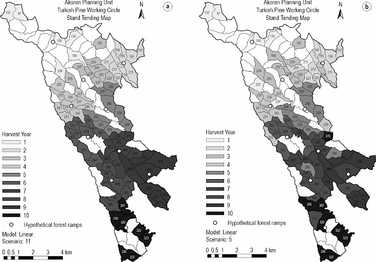
Fig. 3 Stand tending map produced by linear thinning model (a – scenario 11, b – scenario 5)

3.2 Results of Nonlinear Thinning Model

With respect to the NLTM, where now the deviation in the average distance between scheduled compartments and forest ramps was to be minimized, the results were as good as the results from the LTM. Here, a 1 km distance was set as average distance target between scheduled compartments and forest ramps. The total deviation from the target for the distance reference scenario (scenario 11) was 1.17 km (Table 8). The total deviation from the wood flow target was 0 m3 for seven scenarios (scenarios 1, 2, 3, 4, 5, 6 and 7) (Table 8 and 9).When the volume and distance deviations are evaluated together, scenario 3, where the weights were 0.8 for volume and 0.2 for average distance, seemed to have provided the best results. Interestingly, the NLTM provided better scheduled volume results (minor deviations from its target) than the LTM. The average distance between scheduled compartments under scenario 3 ranged from 1.5 km (in year 8) to 2.5 km (in year 1), or 50 to 150% greater than the target value (Table 10). Across all scenarios and for all years, the actual average distance between scheduled compartments and forest ramps indicated that in only one case the results of the NLTM were better than those obtained through the LTM. However, the processing time of the NLTM was much shorter. In order to graphically illustrate the results of the NLTM, the scheduled compartments and forest ramps within each year of scenario 11 (reference for distance goal) and 3 (best results), are noted in Fig. 4.

Table 8 Outcomes achieved by nonlinear thinning model

Table 9 Volume scheduled and deviations from volume target when using NLTM (m3)

Table 10 Actual distance of compartments to ramps and deviations from distance target when using NLTM (km)

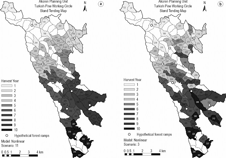
Fig. 4 Stand tending map produced by nonlinear thinning model (a – scenario 11, b – scenario 3)

3.3 Comparison of Actual Stand Tending Plan with Model Results

An intermediate harvest plan (stand tending plan) was prepared by the General Directorate of Forestry (2014). The local forester was responsible for creating thinning blocks on the condition of scheduling annually 1/10th of the planned decadal intermediate allowable cut. Since stand tending blocks were not created in the management plan, we could not fully compare the results of our thinning models with the actual forest management plan data. Therefore, we obtained the actual annual cutting plans for 2014–2018, prepared by local foresters (Pos Forest District Directorate 2017). We reconstituted a 5-year cutting plan table for the study area based on the annual plans (Table 11). However, we were only able to compare the total (and average) distances between the centroids of scheduled compartments within the same thinning block.

Table 11 Actual intermediate harvest plan of the study area (stand tending plan)

Using scenario 5 of the linear model, the average (for 5 years) deviation from annual allowable cut volume was only 0.4 m3, and the average of total distances (for 5 years) between the centroids of scheduled compartments within the same thinning block was 89.6 km (Table 12). Using scenario 3 of the nonlinear model, there was no deviation from annual allowable cut volume in 5 years, and the average of total distances between tended units was 105 km. In the actual plan, the deviations in scheduled volumes over the 5-year period were 660.4 m3 per year. Considering that the average intermediate yield allowable cut is 2,628 m3 per year for the study area, this deviation is noteworthy (25% of the volume target). Further, the distances between the centroids of scheduled compartments in the actual plan totaled 122.2 km. This will result in loss of time and money in the transport of cutting and skidding equipment from one compartment to another, and will also make it difficult to control the harvesting operations.

Table 12 Comparison of actual stand tending plan data with study results

4. Discussion

The contribution of this work has been to illustrate alternative methods for addressing a timber production program conducted in the thinning compartments of a forest district within a government-controlled European/Asian forested landscape. This work expands upon the work of others (e.g., Demirci and Bettinger 2015) to show that a nonlinear method for the development of an intermediate harvest plan can effectively be developed to provide reasonable results that form the basis of a management plan. To model the intermediate harvest plan, consideration was given to the advantages of working in the same terrain, and thus through the recognition of distance to ramps, compartments are often clumped together to create thinning blocks. Further, when preparing annual budgets and planning to meet the market’s needs, forest enterprises desire the annual intermediate harvest yield to be nearly equal each year. However, decision support systems have not been used by the Turkish foresters so far in order to designate the location of the stand tending blocks and to harvest an equal amount of wood every year from the thinning compartments. Thus, as can be seen from the comparison of the study with the actual plan, the volume deviation at the time of implementation can be up to 25% of the average annual allowable cut. Moreover, the distances between scheduled thinning compartments can be more than 100 km, which makes it difficult to control the harvesting operations. Without modeling this problem mathematically, it seems impossible to develop a plan with an equal amount of harvest each year and thinning blocks that are not too far from one another. We have demonstrated a tractable process to develop efficient plans that can be used as guidance to field foresters for implementation of intermediate harvests.

Our stand tending problem (creation of stand tending blocks) is a forest level spatial optimization problem that aggregates compartments. In Scandinavian countries, a commonly modeled aggregation problem is the minimization of the fragmentation of mature forests (Öhman 2000, Öhman and Eriksson 2002). Minimizing older forest fragmentation can be achieved, for example, by having a certain core area for each of the first period and minimizing the difference between the total amounts of old forest and the total amount of core area (Öhman 2000) or maximizing the boundary between adjacent natural old forest stands. In spatial forest planning, minimizing and maximizing operations such as these (not deviations from the target value) are usually performed using mixed-integer programming methods since the integer assumption of decision variable values facilitates tracking adjacent conditions (Bettinger and Chung 2004). When decision variables are assigned continuous real numeric values in a mathematical programming problem, the resulting size of an older forest (or final harvest) is uncertain, since one cannot assume that the partial assignment of activity within one stand touches the partial assignment of activity in another adjacent stand. Unfortunately, when integer or binary decision variables are assumed in a problem formulation, a branch and bound or cutting plane method (or both) problem-solving process is typically employed, which can dramatically increase the computational effort. With a total of 1760 variables, including 20 nonlinear variables and 10 nonlinear constraints, NLTM presents a somewhat more difficult problem than LTM. However, the processing time of the NLTM was much shorter. While it took almost 28 hours to run all 11 scenarios of the LTM, it took only 3 hours, 21 minutes and 50 seconds to run all NLTM scenarios. The longest computing time was 10 hours and 1 minute and 28 seconds (LTM scenario 3).

Ultimately, both models (linear and nonlinear) developed to solve the intermediate harvest problem produced reasonable results both in aggregating thinning compartments and in scheduling equal amounts of harvest volume each year. The models can be further enhanced by including other important management issues, such as road availability, silvicultural priorities, and availability of labour into the objective function or constraints. In incorporating a road system into the planning model, for example, a reduction in road density might be suggested, which may help contribute to improvements in ecological goals. Further, there may exist other silvicultural priorities, such as management actions that would improve forest health, which may contribute to sustainable forest management goals. These may be seen as intermediate activities that can be scheduled alongside the thinnings to assist in meeting wood flow targets. Since sustainable forest management could include economic, ecological, and social goals, the management of forests to minimize large deviations in these factors could become quite complex. If a goal can be quantified, GP seems to be an appropriate technique to address these management issues, rather than representing them as constraints within a management model (Demirci and Bettinger 2015).

The sensitivity of the models described here was assessed by evaluating how the results (harvest volume and distance of compartments to ramps) might change when the weights applied in the objective function varied. One challenge of the planner is to determine the appropriate weights to be applied to the components of the objective function (Demirci and Bettinger 2015), such as seeking the opinion of experts and attempting to find a consensus. The issue of normalization is important when attempting to overcome the incommensurability that occurs when deviational variables are represented by different units (ha, m3, km, etc.). Either normalizing or weighting the values of disparate outcomes in the objective function can place them on common ground. We chose the weighting approach, since each of the outcomes (differences in timber produce from a target and differences in distances between treatments from a target) was expected to approach zero in the ideal case and the closer they were to the ideal, the less need there was to normalize their values, especially when scenarios 9 and 10 are considered (weighting distances by 0.7 or 0.8 and volumes by 0.2 or 0.3). However, the simple summation of different units in an objective function may cause an unintentional bias towards those with a larger magnitude, such as wood flow in our case (as compared to distance to a forest ramp). To overcome this problem, one may have to locate weights that ensure all objectives have roughly the same magnitude in the objective function. Alternatively, normalization constants can be developed through percentage, Euclidean, summation, or zero-one normalization processes (De Kluyver 1979, Masud and Hwang 1981, Wildhelm 1981, Romero 1991, Jones 1995, Tamiz et al. 1998). However, the use of these normalization processes cannot guarantee that the outcomes will be consistent with their goals (Jadidi et al. 2014). Therefore, with regard to the forestry problems described here, this area of investigation is still open.

5. Conclusions

In this study, we described how mixed-integer GP might be used within a Turkish forest management planning system to recognize important issues related to stand tending (intermediate harvests). Our work illustrated a new approach to temporal and spatial scheduling of intermediate yield harvests, which provided an enhancement on previous research related to this management concern. Although the process was accommodated through spreadsheet and manual manipulation of data, decision-makers should evaluate if this is a useful process for thinning planning purposes, and a matrix generator should be developed to solve these (and similar) problems. Alternatively, processes to address these issues within commercial forest planning software might be explored. Further research can be conducted to address the limitations of this study, such as the excessive computer processing time of mixed-integer models that use branch and bound search processes, and the large number of iterations necessary to arrive at the optimal solution. Finally, while this methodology was demonstrated on a relatively small case study landscape, it could be applied to larger problems and different planning units world-wide to assess the temporal and spatial scheduling of forests intermediate planning.

Acknowledgements

This research was funded by the Scientific Research Projects Coordination Unit of the Istanbul University-Cerrahpasa (Project number: 20612). This research was supported by the U.S. National Institute of Food and Agriculture McIntire-Stennis research program (Project number: GEOZ-0195-MS). We would like to thank the officials of the Forest Management Planning Department of the General Directorate of Forestry in Turkey for sharing the management plan data and GIS data of the study area. We also thank the local foresters for sharing the actual silviculture plan of the study area forest.

6. References

Aldea, J., Martínez-Peña, F., Romero, C., Diaz-Balteiro, L., 2014: Participatory goal programming in forest management: An application integrating several ecosystem services. Forests 5(12): 3352–3371. https://doi.org/10.3390/f5123352

Augustynczik, A.L.D., Arce, J.E., da Silva, A.C.L., 2016: Aggregating forest harvesting activities in forest plantations through integer linear programming and goal programming. Journal of Forest Economics 24: 72–81. https://doi.org/10.1016/j.jfe.2016.06.002

Bagdon, B.A., Huang, C.-H., Dewhurst, S., 2016: Managing for ecosystem services in northern Arizona ponderosa pine forests using a novel simulation-to-optimization methodology. Ecological Modelling 324: 11–27. https://doi.org/10.1016/j.ecolmodel.2015.12.012

Bare, B., Anholt, B., 1976: Selecting forest residue treatment alternatives using goal programming, USDA Forest Service, General Technical Report PNW-43. Pacific Northwest Forest and Range Experiment Station, Portland, OR, USA.

Bell, E.F., 1975: Problems with goal programming on a national forest planning unit. In Systems Analysis and Forest Resource Management; Meadows, J., Bare, B., Ware, K., Row, C., Eds.; Society of American Foresters: Bethesda, MD, USA, 119–126 p.

Bertomeu, M., Romero, C., 2001: Managing forest biodiversity: a zero-one goal programming approach. Agricultural Systems 68(3): 197–213. https://doi.org/10.1016/S0308-521X(01)00007-5

Bertomeu, M., Romero, C., 2002: Forest management optimization models and habitat diversity: a goal programming approach. Journal of the Operational Research Society 53(11): 1175–1184. https://doi.org/10.1057/palgrave.jors.2601442

Bettinger, P., Chung, W., 2004: The key literature of, and trends in, forest-level management planning in North America, 1950–2001. International Forestry Review 6(1): 40–50. https://doi.org/10.1505/ifor.6.1.40.32061

Charnes, A., Cooper, W.W., 1961: Management models and industrial applications of linear programming: Vol 1. John Wiley & Sons: New York, NY, USA.

Charnes, A., Cooper, W.W., Ferguson, R.O., 1955: Optimal estimation of executive compensation by linear programming. Management Science 1(2): 138–151. https://doi.org/10.1287/mnsc.1.2.138

Chen, Y.-T., Chang, C.-T., 2014: Multi-coefficient goal programming in thinning schedules to increase carbon sequestration and improve forest structure. Annals of Forest Science 71(8): 907–915. https://doi.org/10.1007/s13595-014-0387-z

Chen, Y.-T., Zheng, C., Chang, C.-T., 2011: 3-level MCGP: An efficient algorithm for MCGP in solving multi-forest management problems. Scandinavian Journal of Forest Research 26(5): 457–465. https://doi.org/10.1080/02827581.2011.578584

De Kluyver, C.A., 1979: An exploration of various goal programming formulations – with application to advertising media scheduling. Journal of the Operational Research Society 30(2): 167–171. https://doi.org/10.1057/jors.1979.30

Demirci, M., Bettinger, P., 2015: Using mixed integer multi-objective goal programming for stand tending block designation: A case study from Turkey. Forest Policy and Economics 55: 28–36. https://doi.org/10.1016/j.forpol.2015.03.007

Diaz-Balteiro, L., Romero, C., 1998: Modeling timber harvest scheduling problems with multiple criteria: an application in Spain. Forest Science 44(1): 47–57. https://doi.org/10.1093/forestscience/44.1.47

Diaz-Balteiro, L., Romero, C., 2003: Forest management optimization models when carbon captured is considered: a goal programming approach. Forest Ecology and Management 174(1–3): 447–457. https://doi.org/10.1016/S0378-1127(02)00075-0

Dress, P.E., 1975: Forest land use planning-an applications environment for goal programming. In Systems Analysis and Forest Resource Management; Meadows, J., Bare, B., Ware, K., Row, C., Eds.; Society of American Foresters: Bethesda, MD, USA, 37–47 p.

Eraslan, İ., 1982: Forest Management, Istanbul University Faculty of Forestry: Istanbul, Turkey.

Field, D.B., 1973: Goal programming for forest management. Forest Science 19(2): 125–135. https://doi.org/10.1093/forestscience/19.2.125

Field, R.C., Dress, P.E., Fortson, J.C., 1980: Complementary linear and goal programming procedures for timber harvest scheduling. Forest Science 26(1): 121–133. https://doi.org/10.1093/forestscience/26.1.121

General Directorate of Forestry, 2014: Ecosystem Based Functional Forest Management Plan of the Akoren Sub-district, General Directorate of Forestry, Ankara, Turkey.

Gómez, T., Hernández, M., Molina, J., León, M.A., Aldana, E., Caballero, R., 2011: A multi objective model for forest planning with adjacency constraints. Annals of Operations Research 190(1): 75–92. https://doi.org/10.1007/s10479-009-0525-4

Hossain, S.M.Y., Robak, E.W., 2010: A forest management process to incorporate multiple objectives: A framework for systematic public input. Forests 1(3): 99–113. https://doi.org/10.3390/f1030099

Hotvedt, J.E., 1983: Application of linear goal programming to forest harvest scheduling. Southern Journal of Agricultural Economics 15(1): 103–108. https://doi.org/10.1017/S0081305200016034

Hotvedt, J.E., Leuschner, W.A., Buhyoff, G.J., 1982: A heuristic weight determination procedure for goal programs used for harvest scheduling models. Canadian Journal of Forest Research 12(2): 292–298. https://doi.org/10.1139/x82-042

Jadidi, O., Zolfaghari, S., Cavalieri, S., 2014: A new normalized goal programming model for multi-objective problems: a case of supplier selection and order allocation. International Journal of Production Economics 148: 158–165. https://doi.org/10.1016/j.ijpe.2013.10.005

Jones, D.F., 1995: The Design and Development of an Intelligent Goal Programming System. PhD Thesis, University of Portsmouth, Portsmouth, UK.

Kahalas, H., Groves, D.I., 1978: Modeling for organizational decision-making: profits vs. social values in resource management. Journal of Environmental Management 6(1): 73–84.

Kangas, J., Pukkala, T., 1992: A decision theoretic approach applied to goal programming of forest management. Silva Fennica 26(3): 169–176. https://doi.org/10.14214/sf.a15645

Kao, C., Brodie, J.D., 1979: Goal programming for reconciling economic, even flow, and regulation objectives in forest harvest scheduling. Canadian Journal of Forest Research 9(4): 525–531. https://doi.org/10.1139/x79-087

Kettani, O., Aouni, A., Martel, J.-M., 2004: The double role of the weight factor in the goal programming model. Computers & Operations Research 31(11): 1833–1845. https://doi.org/10.1016/S0305-0548(03)00142-4

Köse, S., 1986: Possibilities of utilizing operations research methods in planning forest enterprises. PhD Thesis, Karadeniz Technical University, Trabzon, Turkey.

Lindo Systems, Inc. 2016. Lingo 16.0. Lindo Systems, Inc., Chicago, Illinois.

Lyon, G., 1974: Applications of goal programming and accounting for control in the forest industry, Unpublished manuscript. Res. Pap., 53 p. College of Forest Resources, University of Washington, Seattle.

Masud, A.S., Hwang, C.L., 1981: Interactive sequential goal programming. Journal of the Operational Research Society 32(5): 391–400. https://doi.org/10.1057/jors.1981.76

Mısır, M., 2001: Developing a multi-objective model forest management plan using GIS and goal programming (a case study of ormanüstü planning unit). PhD Thesis, Karadeniz Technical University, Trabzon, Turkey.

Mısır, N., Mısır, M., 2007: Developing a multi-objective forest planning process with goal programming: a case study. Pakistan Journal of Biological Sciences 10(3): 514–522. http://dx.doi.org/10.3923/pjbs.2007.514.522

Öhman, K., 2000: Creating continuous areas of old forest in long term forest planning. Canadian Journal of Forest Research 30(11): 1817–1823. https://doi.org/10.1139/x00-103

Öhman, K., Eriksson, L.O., 2002: Allowing for spatial consideration in long term forest planning by linking linear programming with simulated annealing. Forest Ecology and Management 161(1–3): 221–230. https://doi.org/10.1016/S0378-1127(01)00487-X

Porterfield, R.L., 1973: Predicted and potential gains from tree improvement programs – a goal programming analysis of program efficiency. PhD Thesis, Yale University, New Haven, CT, USA.

Porterfield, R.L., 1974: Predicted and potential gains from tree improvement programs: a goal programming analysis of program efficiency, North Carolina State University, School of Forest Resources, Technical Report No. 52, 112 p.

Pos Forest District Directorate, 2017: Annual cutting plans archive of the Pos Forest District Directorate, Adana Forest Regional Directorate, Turkey.

Romero, C., 1991: Handbook of Critical Issues in Goal Programming; Pergamon Press: Oxford, UK.

Romesburg, C.H., 1974: Scheduling models for wilderness recreation. Journal of Environmental Management 2(2): 159–177.

Rustagi, K.P., 1973: Forest management planning for timber production: a goal programming approach. PhD Thesis, Yale University, New Haven, Connecticut.

Schuler, A.T., Meadows, J.C., 1975: Planning resource use on natural forests to achieve multiple objectives. Journal of Environmental Management 3(4): 351–366.

Schuler, A.T., Webster, H.H., Meadows, J.C., 1977: Goal programming in forest management. Journal of Forestry 75(6): 320–324. https://doi.org/10.1093/jof/75.6.320

Silva, M., Weintraub, A., Romero, C., De la Maza, C., 2010: Forest harvesting and environmental protection based on the goal programming approach. Forest Science 56(5): 460–472. https://doi.org/10.1093/forestscience/56.5.460

Tamiz, M., Jones, D., Romero, C., 1998: Goal programming for decision making: an overview of the current state-of-the-art. European Journal of Operational Research 111(3): 569–581. https://doi.org/10.1016/S0377-2217(97)00317-2

United Nations Food and Agriculture Organization, 2016: Global Forest Resources Assessment 2015: How are the world’s forests changing? 2nd ed., FAO: Rome, Italy.

United Nations Food and Agriculture Organization, 2020: Global Forest Resources Assessment 2020 – Main report. FAO: Rome, Italy.

Wildhelm, W.B., 1981: Extensions of goal programming models. Omega 9: 212–214.

Zengin, H., Asan, Ü., Destan, S., Ünal, M.E., Yeşil, A., Bettinger, P., Değermenci, A.S., 2015: Modeling harvest scheduling in multifunctional planning of forests for long term water yield optimization. Natural Resource Modeling 28(1): 59–85. https://doi.org/10.1111/nrm.12057.

© 2021 by the authors. Submitted for possible open access publication under the
terms and conditions of the Creative Commons Attribution (CC BY) license (http://creativecommons.org/licenses/by/4.0/).

Authors’ addresses:

Mehmet Demirci, PhD *

e-mail: mehmetdemirci@yahoo.com

Ministry of Agriculture and Forestry

Beştepe Mahallesi, Alparslan Türkeş Caddesi, No: 71

06560, Yenimahalle, Ankara

TURKEY

Prof. Ahmet Yeşil, PhD

e-mail: ayesil@istanbul.edu.tr

Istanbul University-Cerrahpasa

Faculty of Forestry

34473, Istanbul

TURKEY

Prof. Pete Bettinger, PhD

e-mail: pbettinger@warnell.uga.edu

University of Georgia

Warnell School of Forestry and Natural Resources

30602, Athens, GA

UNITED STATES

* Corresponding author

Received: June 10, 2020

Accepted: September 13, 2021

Original scientific paper