Design of a Six-Swing-Arm Wheel-Legged Chassis for Forestry and Simulation Analysis of its Obstacle-Crossing Performance
doi: 10.5552/crojfe.2023.1373
volume: 44, issue:
pp: 16
- Author(s):
-
- Gao Yaoyao
- Zeng Zechen
- Kan Jiangming
- Article category:
- Original scientific paper
- Keywords:
- six-swing-arm wheel-legged chassis for forestry, coordinate transformation, kinematic model, ADAMS/Simulink co-simulation
Abstract
HTML
Obstacle-crossing performance is an important criterion for evaluating the power chassis of forestry machinery. In this paper, a new six-swing-arm wheel-legged chassis (SWC&F) is designed according to the characteristics of forest terrain, using herringbone legs to control the ride comfort and stability of the chassis in the process of crossing obstacles. First, the kinematic model of the SWC&F is established, the coordinate analytical expression of each wheel centre position is derived, and the swing angle range of each wheel leg of the chassis is calculated according to the installation position of the hydraulic cylinder. Next, the control model of the system is constructed, and the obstacle-crossing performance of the SWC&F is analyzed by ADAMS/Simulink co-simulation using the PID control method and conventional control method, respectively. The results show that the maximum obstacle crossing height of the SWC&F can reach 411.1 mm, and the chassis with PID control system has good dynamic response characteristics and smooth motion, which meets the requirements of forest chassis obstacle crossing design. The study can provide the foundation for the practical laws of the physical prototype of the forest vehicle chassis.
Design of a Six-Swing-Arm Wheel-Legged Chassis for Forestry and Simulation Analysis of its Obstacle-Crossing Performance
Yaoyao Gao, Zechen Zeng, JiangMing Kan
Abstract
Obstacle-crossing performance is an important criterion for evaluating the power chassis of forestry machinery. In this paper, a new six-swing-arm wheel-legged chassis (SWC&F) is designed according to the characteristics of forest terrain, using herringbone legs to control the ride comfort and stability of the chassis in the process of crossing obstacles. First, the kinematic model of the SWC&F is established, the coordinate analytical expression of each wheel centre position is derived, and the swing angle range of each wheel leg of the chassis is calculated according to the installation position of the hydraulic cylinder. Next, the control model of the system is constructed, and the obstacle-crossing performance of the SWC&F is analyzed by ADAMS/Simulink co-simulation using the PID control method and conventional control method, respectively. The results show that the maximum obstacle crossing height of the SWC&F can reach 411.1 mm, and the chassis with PID control system has good dynamic response characteristics and smooth motion, which meets the requirements of forest chassis obstacle crossing design. The study can provide the foundation for the practical laws of the physical prototype of the forest vehicle chassis.
Keywords: six-swing-arm wheel-legged chassis for forestry, coordinate transformation, kinematic model, ADAMS/Simulink co-simulation
1. Introduction
Forest resources are the basis of human social development and a precious resource for society (Gao et al. 2021, Oliveira-Nascimento et al. 2021). All countries attach great importance to the conservation and utilization of forest resources (Sampietro et al. 2022). The application of forestry fire prevention and forestry exploration will be especially critical when faced with such a vast land area and a large number of forest resources (Couceiro and Portugal 2018). The quality of forestry equipment will directly affect the sustainable development of the forestry industry. To achieve the goal of mechanization, automation, and intelligentization of forestry equipment, the first thing to be solved is the problem of equipment chassis (McConnell 2021). Due to its operating environment, the forestry equipment chassis is more complex compared to ordinary engineering vehicles, and has higher requirements for barrier/obstacle crossing performance (Zhu and Kan 2016).
According to the different travelling mechanisms, forestry equipment chassis can be classified into three types: wheeled chassis, tracked chassis, and legged chassis (Zhu et al. 2018). The performance of tracked chassis has been studied by a large number of scholars. Sun S.F. et al. (2021) developed an LY1352JP tracked vehicle-based on complex terrain and simulated the vehicle performance using RecurDyn software. The results show that the maximum width across the trench and the vertical crossing height of the vehicle are 1.35 m and 0.45 m, respectively. Sun Y.X. et al. (2020) developed a tracked harvester flattening chassis that adjusts the posture of the chassis using hydraulic cylinder travel. The chassis has a maximum ground clearance adjustment range of 140 mm and a side lean adjustment range of ±5.17°. The tracked chassis has a better barrier crossing performance and can be used for field operations without roads (Zemanek and Neruda 2021). However, the tracked chassis has a large contact area with the ground and causes more damage to surface vegetation during travel and steering. At the same time, tracked vehicles are usually transported on special flatbed trucks by road and forest roads, which is a cumbersome process (Kormanek and Dvorak 2021).
Although conventional wheeled vehicles operate efficiently and cause minimal damage to forest soils, movement in rough terrain can be limited by movement through forested areas (Sun, Li, et al. 2020). Therefore, legged structures have been proposed. Compared to conventional mechanisms, the legged chassis is highly adaptable to the terrain and allows for multiple degrees of freedom of movement (Li et al. 2019). However, the relatively complex structure and high control complexity limit its mobility in rough terrain (Qu et al. 2017).
The wheel-leg type combines the advantages of wheeled and legged chassis, which is the most widely used method on uncertain surfaces today (Li and Kang 2020). Ahtohob et al. (2017) proposed a kinematic model of a three-point wheel-legged robot and built the model in SolidWorks software. Based on the Newton-Euler equations, inverse dynamics equations describing the motion of the robot in the walking mode were developed and simulated in SimMechanics and MATLAB, but they are less stable compared to the six-legged robot. Sun Z.B. et al. (2022) proposed a new articulated wheel-legged forestry chassis, based on a flexible kinematic model of the rotational screw theory, to analyze the adjustment capability characteristics of the chassis. Due to its complex degrees of freedom and posture, the control system is complicated, making it impossible to achieve the ideal movement position. On this basis, this paper proposes a new SWC&F. Its kinematic model is established using the Denavit-Hartenberg Matrix parameter method, and the swing angle range of each wheel leg is determined according to the installation position of the hydraulic cylinder. Finally, the smoothness of crossing obstacles was analyzed by a joint ADAMS/Simulink simulation. This provides a theoretical basis for the development and application of intelligent harvesting chassis for forestry machinery.
2. Materials
2.1 Structural Design of SWC&F
2.1.1 Structural Design
Under the complex conditions of the forest operation environment, the working platform is required to have good obstacle-crossing and mobility performance to maintain the ideal travel efficiency on the highly uneven ground (Routa et al. 2020). Therefore, this study combines the traditional forestry chassis with the articulated swing-arm vehicle mechanism to propose a new SWC&F. Its structure is mainly composed of wheels, frame, front-wheel legs, herringbone wheel legs, rear-wheel legs and steering mechanism, as shown in Fig. 1. The front frame is fixedly connected to the rear frame. The drive form of the chassis is all-wheel drive, and the power output is transmitted directly to each wheel to ensure the dynamics of the chassis. Through the telescopic action of the hydraulic cylinder, the front wheel leg can do pitching movement around the articulation point, while the herringbone wheel leg can do rotating movement around the articulation point to achieve the maximum vertical obstacle crossing height.
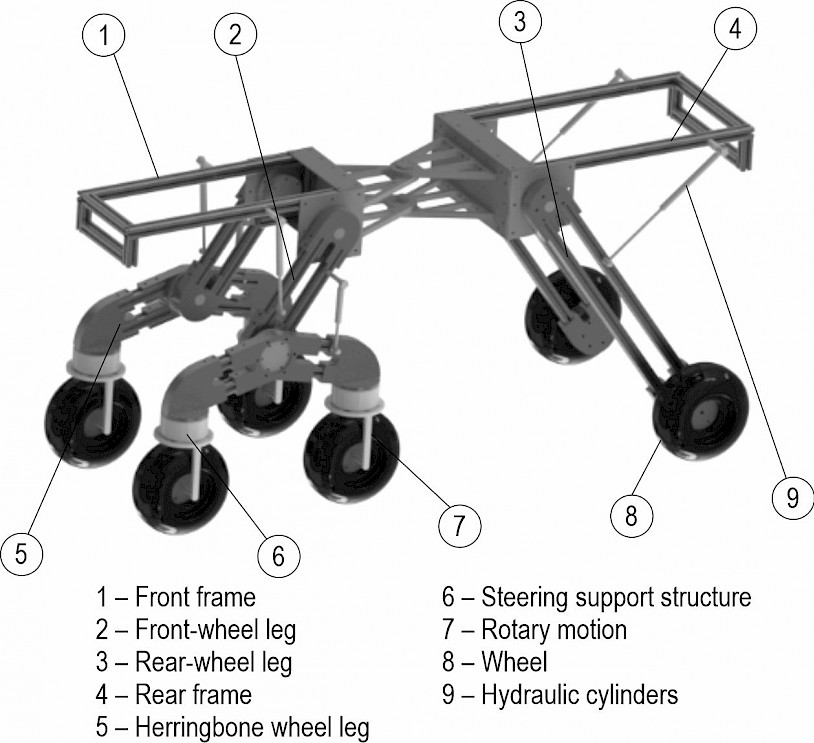
Fig. 1 Structure of SWC&F
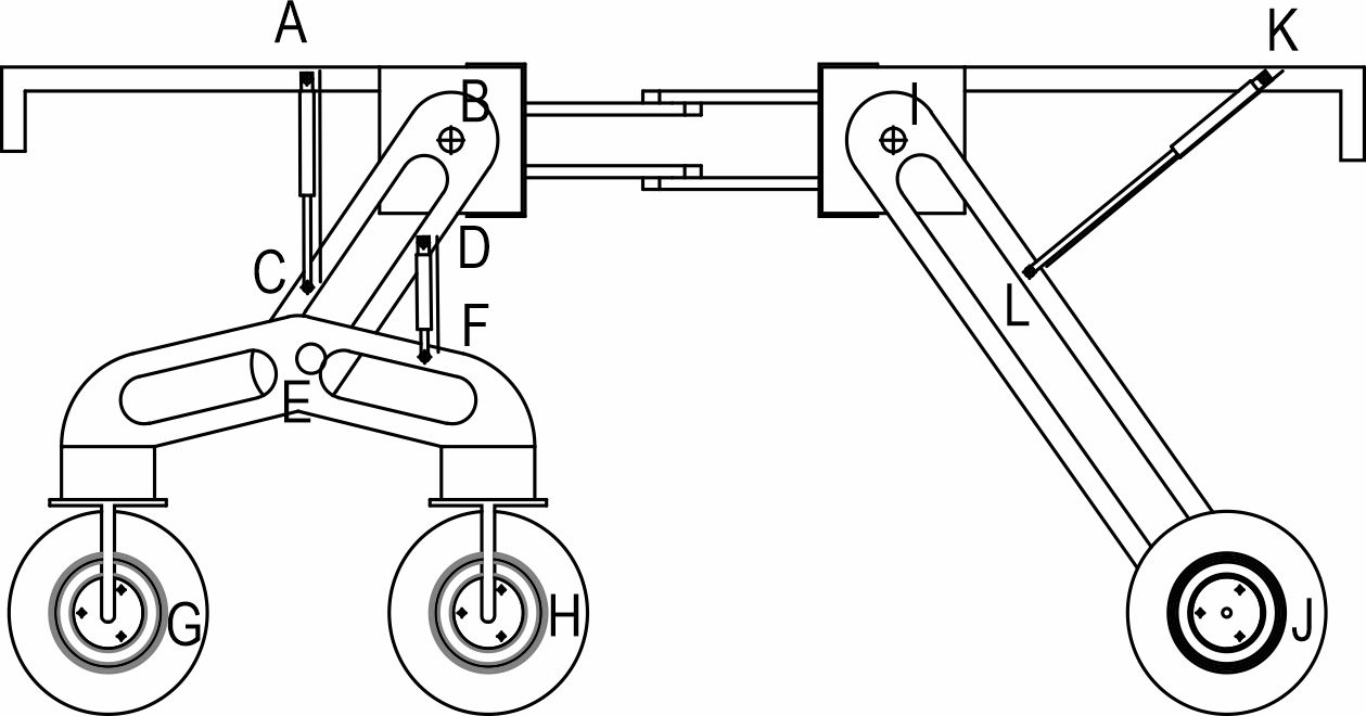
Fig. 2 Hydraulic cylinder installation position
2.1.2 Hydraulic Cylinder Installation Locations
As shown in Fig. 2, the relationship between the swing angle and the length of the hydraulic cylinder can be obtained according to the cosine theorem as follows:
 (1)
(1)
The range of variation of ∠ABC, ∠DEF and ∠LIK is adjusted according to the range of values of LAC, LDF and LKL, where LAB=267.42 mm, LBC=348.5 mm, LDE=295.3 mm, LEF=217.48 mm, LIL=321.25 mm and LIK=644.21 mm.
2.2 Kinematic Model Analysis of SWC&F
2.2.1 Coordinate System of SWC&F
The SWC&F is composed of four relatively independent single wheel legs, which are required to cooperate with each other to complete their functions in the driving process. A fixed coordinate system x0y0z0 is established at the midpoint of the articulation point between the front frame and the two front wheel legs, and the 12 centres of rotation of the chassis swing arm (swing arm articulation axis and wheel axis) are used as the origin to establish the coordinate system, as shown in Fig. 3.
Where:
The vertical distance between the coordinate system of articulation points 1 & 2 and the 0-based coordinate system is b1=b2=238 mm. The vertical distance between the articulation points 9 & 10 and the 0-based coordinate system is b3=b4=315 mm. The length of the front wheel leg is a1=a2=457 mm, the length of the herringbone wheel leg is a3=a4=530 mm, and the length of the rear wheel leg is a5=a6=977 mm. The distance between the 0-based coordinate system and the midpoint of the rear wheel leg articulation point is L1=759 mm. Table 1 shows the linkage parameters of the SWC&F.
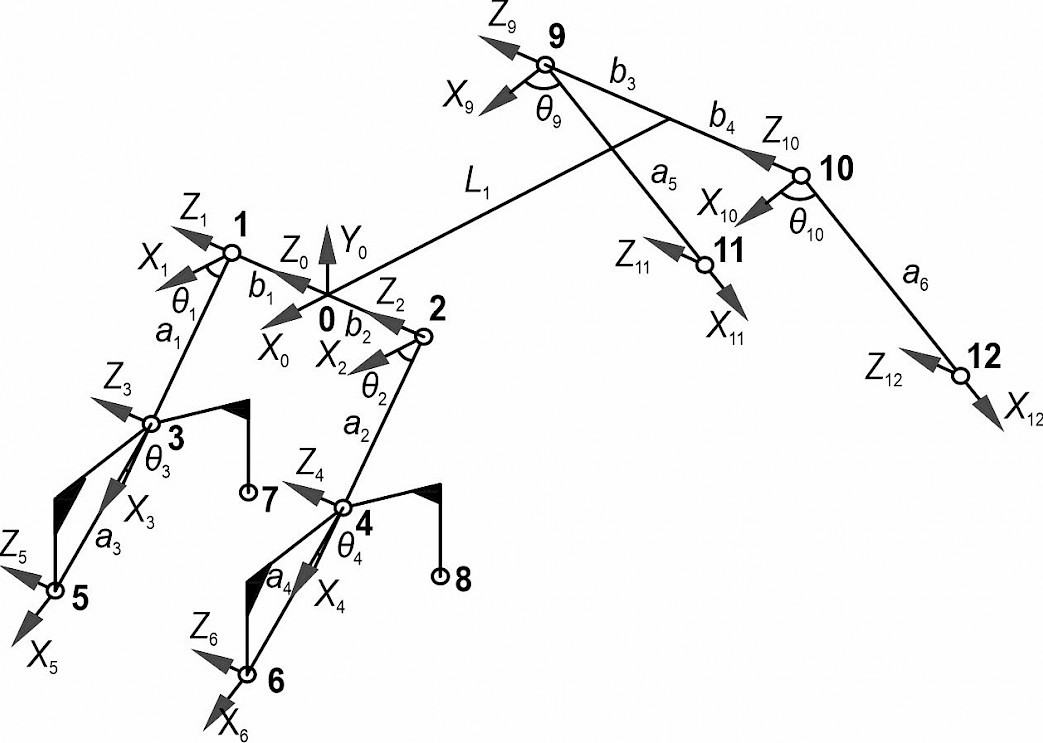
Fig. 3 Coordinate system of SWC&F
Table 1 Linkage parameters of SWC&F
|
Joint i |
αi, ° |
ai, mm |
di, mm |
θi, ° |
|
1 |
0 |
0 |
b1 |
0 |
|
3 |
0 |
a1 |
0 |
-θ1 |
|
5 |
0 |
a3 |
0 |
θ3 |
|
2 |
0 |
0 |
-b2 |
0 |
|
4 |
0 |
a2 |
0 |
-θ2 |
|
6 |
0 |
a4 |
0 |
θ4 |
|
9 |
0 |
L1 |
b3 |
0 |
|
11 |
0 |
a5 |
0 |
-θ9 |
|
10 |
0 |
L1 |
-b4 |
0 |
|
12 |
0 |
a6 |
0 |
-θ10 |
2.2.2 Kinematic Equation of Front-Wheel Leg
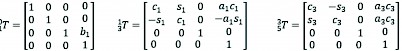
For the left front-wheel leg of the SWC&F in this study, the coordinate transformationmatrix of each joint is shown as follows:
 (2)
(2)
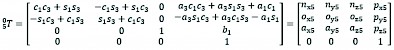
For simplicity, and . By multiplying the coordinate transformation matrices , the equation of motion of the wheel centre 5 is obtained as follows:
 (3)
(3)
According to the coordinate transformation relationship, can be expressed as:
 (4)
(4)
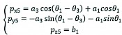
The corresponding coordinates of wheel centre 5 can be obtained as follows:
 (5)
(5)
Similarly, the coordinates of wheel centre 6 can be obtained as follows:
 (6)
(6)
2.2.3 Kinematic Equation of Rear-Wheel Leg
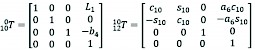
For the right rear-wheel leg of the SWC&F in this study, the coordinate transformation matrix of each joint is shown as follows:
 (7)
(7)
The kinematic equation of the wheel centre 12 can be calculated as:
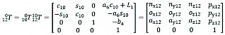 (8)
(8)
The corresponding coordinates of wheel centre 12 are:
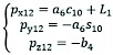 (9)
(9)
Equivalently, the corresponding coordinates of the wheel centre 11 can be obtained as:
 (10)
(10)
2.3 Inverse Kinematic Analysis of SWC&F
2.3.1 Study on Inverse Kinematics of Front-Wheel Leg
From Eq. (4) , and are constants. The equation of the function with joint variables is as follows:
 (11)
(11)
The angle of posture is obtained:
 (12)
(12)
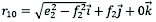
As shown in Fig. 4(a), the vector equation of the wheel centre 5 in the coordinate system 3 is:
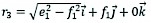 (13)
(13)
Where:
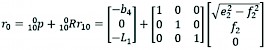
As shown in Fig. 4(b), the coordinates of the wheel centre 5 in the coordinate system 1 can be expressed as:
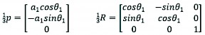 (14)
(14)
 (15)
(15)
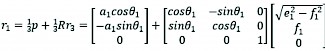
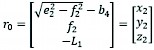
so:
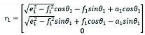 (16)
(16)
The transformation of the wheel centre 5 into the 0 base coordinate system can be expressed as follows:
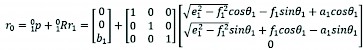 (17)
(17)
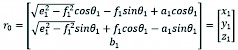 (18)
(18)
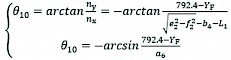
The distance of wheel centre 5 from the 0 base coordinate at the initial position is 792.4 mm, so the relationship equation between the front wheel leg position angle and the crossing height is as follows:
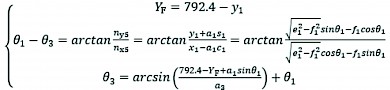 (19)
(19)
Where:
YF Obstacle crossing height, mm.
2.3.2 Study on Inverse Kinematics of Rear-Wheel Leg
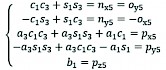
The functional equation with rear-wheel leg joint variables can be derived from Eq. (8) as follows:
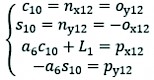 (20)
(20)
As shown in Fig. 4(c), the vector equation of the wheel centre 12 in the base coordinate system 10 is:
 (21)
(21)
Where:
In the same way, the equation of the wheel centre 12 in the 0-based coordinate system can be obtained as follows:
 (22)
(22)
 (23)
(23)
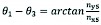
The relationship equation between the rear wheel leg position posture angle and the crossing obstacle height can be obtained:
 (24)
(24)
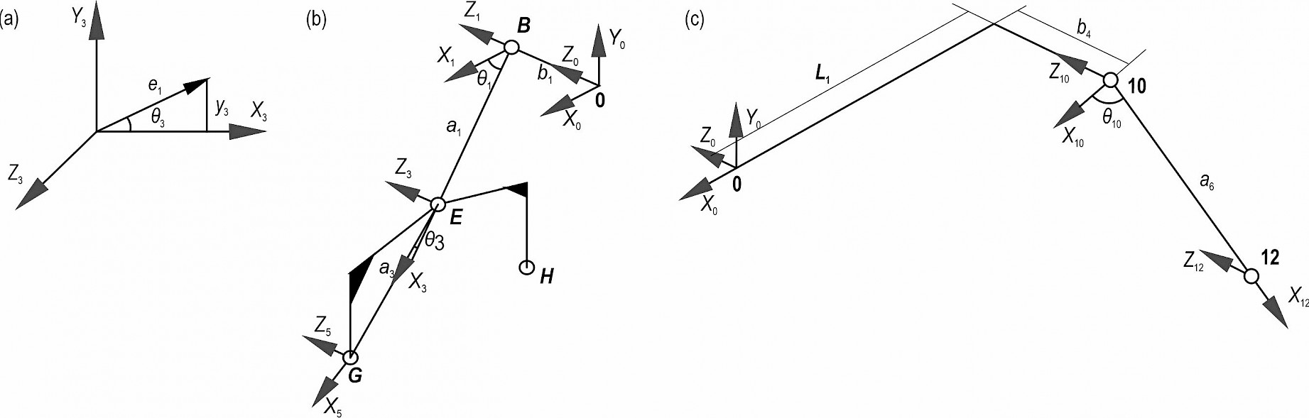
Fig. 4 Converted coordinate system
2.4 Crossing Obstacle Characteristics Analysis of SWC&F
As shown in Fig. 5, the obstacle-crossing process of the SWC&F can be divided into three stages: herringbone front-wheel leg active obstacle-crossing, herringbone rear-wheel leg rear active obstacle-crossing and rear-wheel leg active obstacle-crossing. Herringbone wheel leg active barrier crossing is achieved through the cooperative movement of the front-wheel leg and herringbone wheel leg, while the rear wheel leg crossing is achieved through the separate control of the swing of this wheel leg.
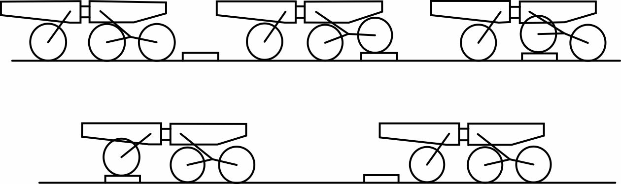
Fig. 5 Diagram of SWC&F crossing process
2.4.1 Analysis of Front-Wheel Obstacle Crossing Characteristics
For the analysis of the maximum displacement over the barrier in the y-axis direction of the front leg, the lifting process of the herringbone leg in the vertical direction in the base coordinate system is obtained according to its swing arm motion. As shown in Fig. 6, the installation angle of point A in the front wheel leg is 22.5°, the installation angle of point C is 9.9°, the installation angle of point D is 11.7°, and the installation angle of point F is 130.93°. It is obtained that:
 (25)
(25)
As shown in Fig. 6, the front wheel leg hydraulic cylinder AC forms a triangle ABC with the front frame and front wheel leg, which is the herringbone wheel leg front wheel crossing mechanism(THFW&M). When the actuator ACmax=350 mm, the result is cos∠ABC=0.38, so θ1max=55.1°. Similarly, when the hydraulic cylinder ACmin=250 mm, the result is cos∠ABC=0.70, so θ1min=33.0°. The corresponding angle of rotation changes from 55.1° to 33.0° when the hydraulic cylinder AC changes from the maximum stroke to the minimum stroke.
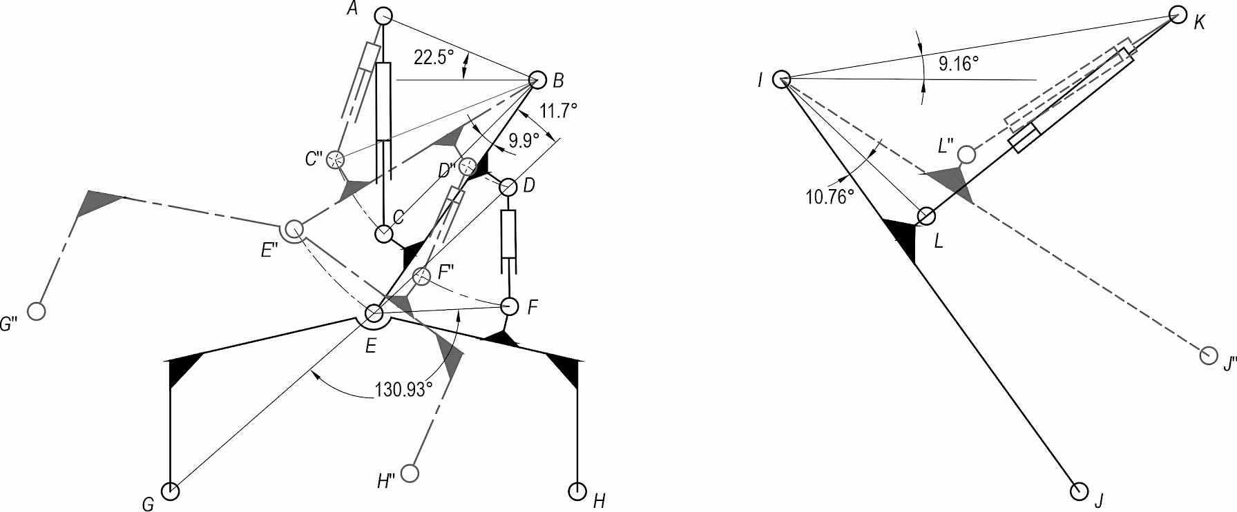
Fig 6. Schematic diagram of the leg swing arm
The hydraulic cylinder DF forms a triangle DEF with the front-wheel leg and herringbone wheel leg, which is the herringbone wheel leg rear-wheel crossing mechanism(THRW&M). When the hydraulic cylinder DFmax=250 mm, it is obtained that θ3max=18.53° . Similarly, when the hydraulic cylinder DFmin=175 mm, it is obtained that θ3min=–0.5° . Namely, when the maximum stroke of the hydraulic cylinder DF changes to the minimum stroke, the corresponding angle of rotation changes from 18.53° to –0.5°.
As shown in Fig. 3, the front wheel leg is in the initial position with θ1=55°, θ3=2.95°, and the initial position of the chassis base coordinate system is 792.4 mm from the ground. When the front-wheel leg crosses the obstacle, θ1 takes the minimum value of 33.0° and θ3 takes the maximum value of 18.53°, which can make the front wheel leg reach the maximum value in the crossing direction. The relationship curves with θ1 and θ3 are shown in Fig. 7(a).
 (26)
(26)
The maximum absolute vertical crossing height is obtained as follows:
 (27)
(27)
2.4.2 Analysis of Rear-Wheel Obstacle Crossing Characteristics
As shown in Fig. 6, the mounting angle of point K is 9.16° and the mounting angle of point L is 10.76°. It can be obtained that:
 (28)
(28)
The hydraulic cylinder KJ forms a triangle PJK with the rear frame and rear-wheel leg, which is the rear wheel leg crossing mechanism (TRW&M). When the hydraulic cylinder KJ stroke changes from 550 mm to 350 mm,∠KIL changes from 58.67° to 16.2°, then θ9 changes from 119.73° to 162.2°, and the change curve is shown in Fig. 7(b). The right rear-wheel leg can be obtained to reach the maximum value of p in the direction of crossing the barrier:
 (29)
(29)
Then the maximum vertical obstacle crossing height of the right rear wheel leg in the y-direction is:
 (30)
(30)
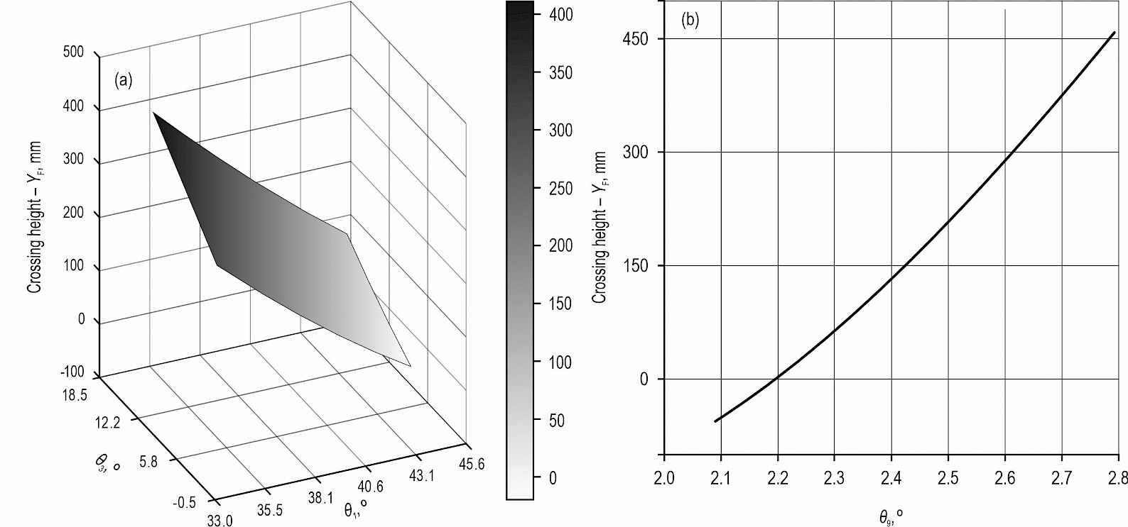
Fig. 7 Relationship curve between wheel leg position angle and obstacle crossing height
3. Methods
3.1 Mathematical Modelling of Control System
Þ Proportional valve electromagnet model
The proportional electromagnet voltage balance equation is:
 (31)
(31)
Where:
ui proportional electromagnet voltage, V
L coil inductance, H
R proportional electromagnet internal resistance, Ω
i coil current, A
t time, s.
The kinetic equation of the solenoid is shown as follows:
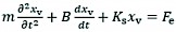 (32)
(32)
Where:
M mass of armature assembly, kg
B damping factor, N/m2
Ks spring stiffness of armature assembly, N/m
Fe electromagnetic suction force, N
xv valve core displacement, m.
The equation of the suction force of the electromagnet in the working stroke is:
 (33)
(33)
Where:
KI current-force conversion coefficient, N/A
Ky displacement-force conversion coefficient, N/m.
A Laplace variation of Eq. (31–33) is obtained as follows (Cristofori and Vacca 2012):
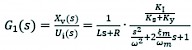 (34)
(34)
 (35)
(35)
Where:
ωm proportional electromagnet intrinsic frequency, rad/s
ξm damping ratio factor of electromagnetic iron.
Þ Proportional valve-controlled hydraulic cylinder model
The linearized flow equation of the proportional valve is:
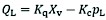 (36)
(36)
Where:
QL flow rate of proportional valve
Kq proportional valve flow gain coefficient
Xv proportional valve spool displacement, m
Kc flow pressure coefficient
pL load pressure drop, Pa.
The hydraulic cylinder flow continuity equation is described as follows:
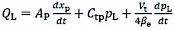 (37)
(37)
Where:
Ap load flow equivalent area of leveling hydraulic cylinder, m2
xp piston displacement of hydraulic cylinder, m
Ctp total hydraulic leakage coefficient
Vt total volume of inlet and returns side of hydraulic cylinder, m3
βe effective volume elastic modulus of fluid, Pa.
The piston force equilibrium equation is:
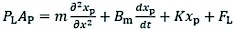 (38)
(38)
Where:
M total mass of piston and load converted to piston, kg
Bm viscous damping coefficient of piston and load, N/m2
K load spring stiffness on piston, N/m
FL load force acting on piston, N.
Since the system has no elastic load, the load spring stiffness on the piston K=0. Assuming that (cylinder inherent frequency, rad/s), (hydraulic cylinder damping ratio), the Laplace transform of Eq. (36–38) can be obtained as follows(Thomas et al.):
 (39)
(39)
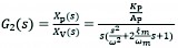
Þ Wheel leg structure transfer function
According to Eq. (2, 26, 29), the displacement of the hydraulic cylinder and the rotation angle of the wheel leg is approximately linear. So the transfer function of the wheel-leg mechanism is:
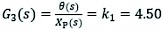 (40)
(40)
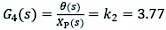 (41)
(41)
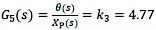 (42)
(42)
Where:
G3(s), G4(s) transfer functions corresponding to front wheel crossing mechanism and rear wheel overrun mechanism of herringbone wheel leg, respectively
G5(s) transfer function corresponding to rear-wheel leg crossing mechanism.
Þ Amplifier transfer function
The circuit part is regarded as an amplifier with a small-time constant, often as a proportional link, so the transfer function of the amplifier is:
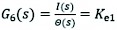 (43)
(43)
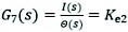 (44)
(44)
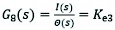 (45)
(45)
Where:
G6(s) and G7(s) - amplifier transfer functions of front wheel crossing mechanism and rear wheel crossing mechanism of herringbone wheel leg, respectively
G8(s) amplifier transfer function of rear wheel leg crossing mechanism.
3.2 System stability analysis
To ensure the stability of the control system, a stability analysis of the system is required to determine the magnitude of the system gain. From the control theory, it is known that the system has stable output, and its amplitude margin and phase margin need to satisfy both the following conditions:
 (46)
(46)
Using Eq. (47) to correct the open-loop gain, it is obtained that the THFW&M , the THRW&M , and the TRW&M , which meet the system stability requirements. The amplifier coefficients Ke1, Ke2, and Ke3 can be inverted.
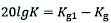 (47)
(47)
Where:
Kg1 original system amplitude margin
Kg desired system amplitude margin.
According to the control system model parameters (Table 2.), the open-loop transfer function of the THFW&M can be obtained as follows:
 (48)
(48)
THRW&M:
 (49)
(49)
TRW&M:
 (50)
(50)
Table 2 Control system model parameters
|
Parameters |
Values |
|
Armature quality m/kg |
0.5 |
|
Electromagnetic force conversion factor Ki/(m·(s·A)-1) |
192.5 |
|
Force conversion factor Ky/(N·m-1) |
570 |
|
Armature assembly spring stiffness Ks/(N·m-1) |
1×10⁴ |
|
Proportional valve electromagnet internal resistance R/Ω |
30 |
|
Proportional valve electromagnet Inductance L/H |
6.6×10⁻² |
|
Electro-hydraulic proportional valve damping ratio ζm |
0.69 |
|
Proportional valve flow rate gain Kq |
2.4 |
|
Total flow pressure coefficient Kce |
4.5×10⁻¹² |
|
Effective volume modulus of elasticity βe |
7×10⁸ |
|
Piston of THFW&M and its load mass m1/kg |
80 |
|
Piston of THRW&M and its load mass m2/kg |
65 |
|
Piston of TRW&M and its load mass m3/kg |
150 |
|
Load flow equivalent area of THFW&M Ap1/m2 |
3.75×10⁻³ |
|
Load flow equivalent area of THRW&M Ap2/m2 |
8.0×10⁻⁴ |
|
Load flow equivalent area of TRW&M Ap3/m2 |
5.1×10⁻³ |
|
Total volume of hydraulic cylinder of THFW&M Vt1/m3 |
6.0×10⁻⁴ |
|
Total volume of hydraulic cylinder of THRW&M Vt2/m3 |
7.5×10⁻⁴ |
|
Total volume of hydraulic cylinder of TRW&M Vt3/m3 |
9.0×10⁻⁴ |
4. Result
For the new forestry crossing chassis designed in this paper, the key of the control strategy is to realize the independent movement of the wheel and leg according to the height of the obstacle. The rotation angle of the wheel-leg joint is changed by the hydraulic cylinder stroke, and the smoothness of the obstacle crossing process is investigated by the joint simulation of ADAMS/Simulink (Wu et al. 2017).
4.1 State Variables
As shown in Fig. 8, the input state variable of the structure during the chassis crossing is the amount of change in the stroke of the six hydraulic cylinders, and the output variable is the rotation angle of the wheel-leg joints. In the figures, inputs 1, 2, 3, 4, 5 & 6 represent the amount of stroke change of the wheel leg hydraulic cylinder, and outputs 1, 2, 3, 4, 5 & 6 represent the rotation angle of the wheel leg joint.
4.2 Control crossing obstacles
The obstacle with a height of 300 mm was created in ADAMS software (Li and Kang 2020), and the rolling resistance coefficient of the designed wheel road surface was 0.025. Based on the PID control strategy shown in Fig. 9, the control block diagram shown in Fig. 10 is created in Simulink. The stroke variation of the hydraulic cylinder is adjusted by a PID controller, which is fed to the actuator (ADAMS) to obtain the rotation angle of the wheel-leg joint. Through the negative feedback adjustment function, the rotation angle of the wheel-leg joint is compared with the target rotation angle to reduce the error and complete the whole closed-loop control process. According to Eq. (19), when the hydraulic cylinders AC and DF are moving at the same speed simultaneously, the optimal solution using Matlab is θ1=36.58° and θ2=12.05°. The simulation parameters are set as follows: the vehicle speed is 3r/s and the simulation time is 11 s.
In the process of obstacle crossing, the oscillation amplitudes of the chassis mass centre in X, Y and Z, as well as the force change curves of the front wheels, middle wheels and rear wheels were measured before and after optimization by PID control.
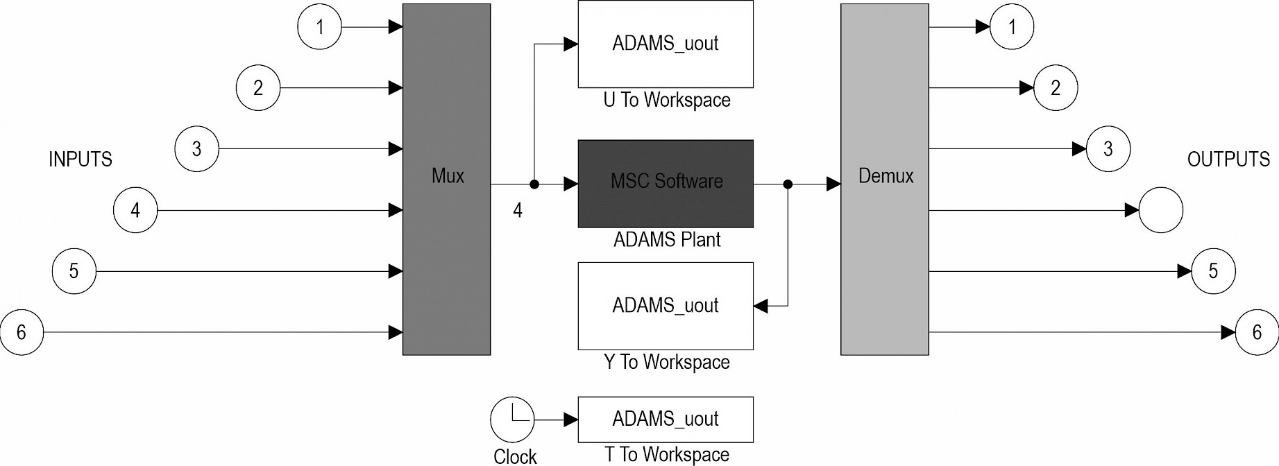
Fig. 8 ADAMS system
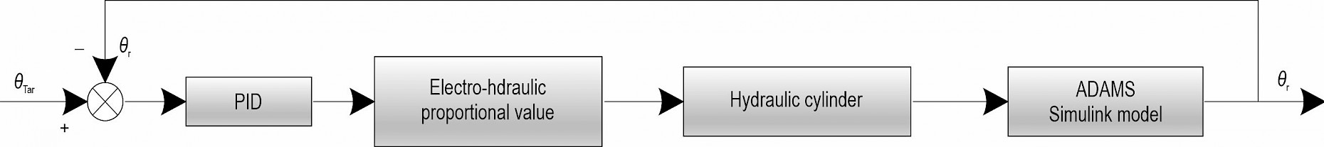
Fig. 9 Control Strategy
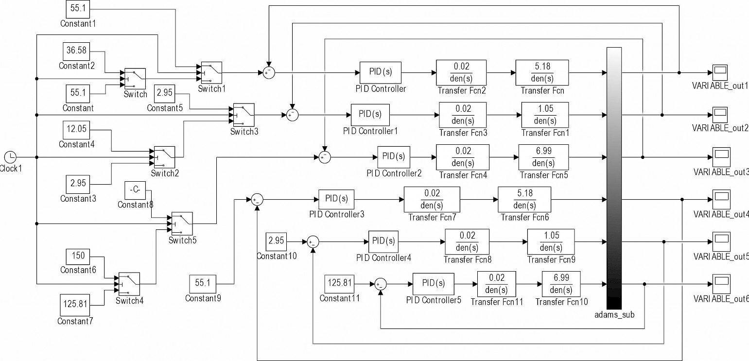
Fig. 10 Control Block Diagram
In the practical application of engineering, the PID controller has the characteristics of simple structure, stable operation and easy adjustment (Yadav and Gaur 2016). This paper involved a simple control system with well-defined parameters to be controlled. Therefore, a simple and effective PID controller is used. The parameters of the PID controller were determined by the decay curve method (Zhou et al. 2019), and the results are shown in Table 3.
Table 3 PID parameter values
|
Kp |
Ki |
Kd |
|
|
THFW&M |
12.45 |
0.0072 |
0.0024 |
|
THRW&M |
10.39 |
0.0102 |
0.0034 |
|
TRW&M |
8.43 |
0.0108 |
0.0036 |
4.3 Simulation results
Fig. 11 and Fig. 12 show the crossing movement of the SWC&F before and after optimization by PID control, respectively. Simulation results show that the chassis without PID control optimization oscillates significantly during obstacle crossing, while the chassis with PID control optimization can cross the obstacle smoothly and smoothly.
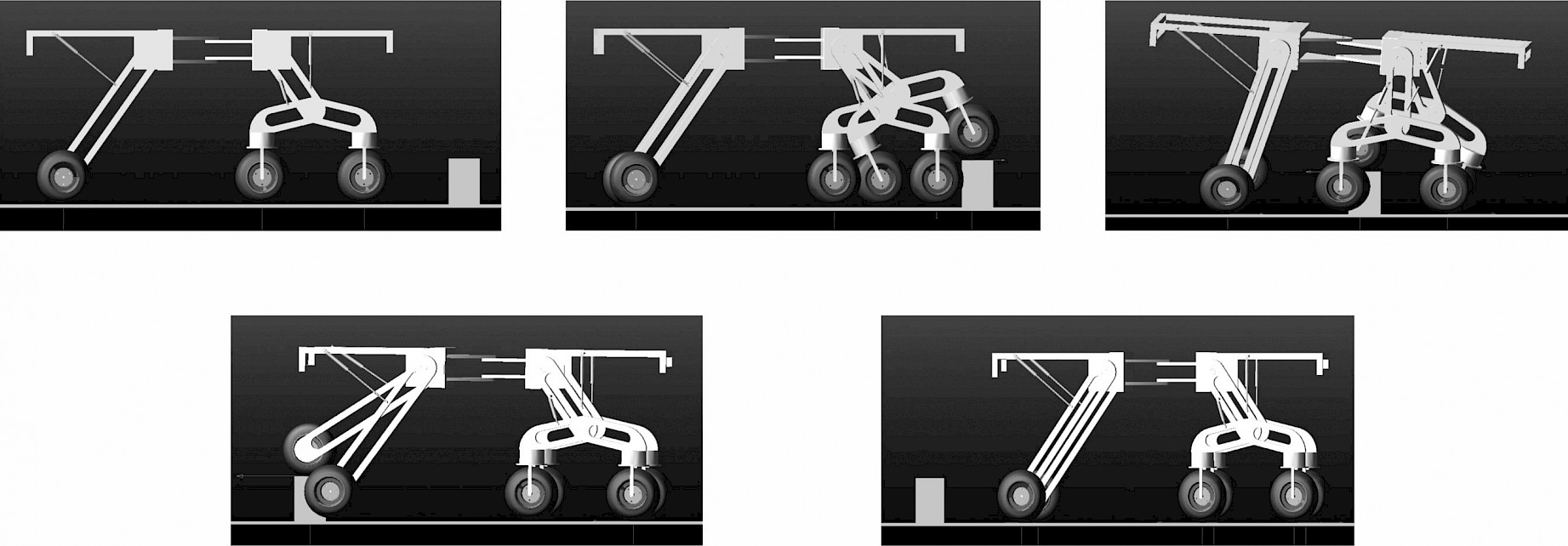
Fig. 11 Schematic diagram of simulation process without PID control of chassis obstacle crossing
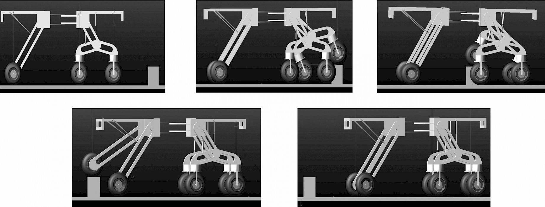
Fig. 12 Schematic diagram of PID controlled chassis obstacle crossing simulation process
5. Discussion
Fig. 13 shows the displacement curve of the barycenter of the SWC&F along the Y direction during the obstacle crossing process before and after PID optimization. It can be seen from the figure that the front wheel of the chassis starts to overcome obstacles at approximately 2.5 s, and the centre of mass position fluctuates and tends to be stable. The response time is 0.25 s without PID optimization. After adding PID control, the response time is 0.11 s and the speed is increased by 56%. At 5.5 s, the front wheel has passed the obstacle, and the middle wheel is beginning to cross the obstacle. The adjustment of the leg position and orientation angle of each wheel makes the chassis tend to be stable, and the mass position of the chassis centre is raised. At approximately 8 s, the front frame of the chassis has passed the obstacle, and the rear frame is ready to pass the obstacle. At 8.5 s, the rear wheel is beginning to overcome the obstacle, and the mass position of the chassis centre also changes slightly afterwards. After 10 s, the entire chassis has been completed and smoothly passed the obstacle. The fluctuation amplitude of the mass centre of the classis is approximately 80 mm without PID control, while the mass centre of the chassis controlled by PID is approximately 50 mm. When there is fluctuation, the chassis optimized by PID control can quickly adjust to the stable state, requiring approximately half of the pre-optimal response time.
Fig. 14(a) and Fig. 14(b) are the swing angle changes of the frame in X and Z directions during the obstacle crossing process of the SWC&F before and after PID optimization. It can be seen from the figure that the amplitude of the swing of the front chassis frame in the X and the Z directions is approximately 9° and 5° respectively, and the frame swings sharply. After using PID control optimization, the swing range of the chassis frame in the X direction is within 2°, and the optimization range is 77.78%. The swing amplitude in the Z direction is also within 2°, and the optimized amplitude is 60%.
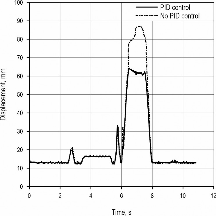
Fig. 13 Mass centre displacement curve of chassis in Y direction before and after PID control
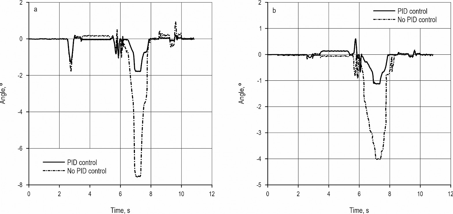
Fig. 14 Swing angle of chassis mass
Fig. 15(a) and Fig. 15(b) show the force curves for the front, middle and rear wheels of the six-wheel swing-arm wheel-leg chassis without and with PID control, in the process of obstacle crossing, respectively. It can be seen from the figure that the chassis optimized by PID control will have a large force when any one of the wheels becomes obstacle-free. Further, the adhesion between the wheel and the road surface is good. Compared with the original model, it has a larger effective driving force and good adhesion.
6. Test Verification
The maximum height obstacle crossing test for the SWC&F was carried out in ADAMS software by creating an obstacle with a height of 411.1 mm and the rolling resistance coefficient of the designed wheel road surface of 0.025. The simulation parameters are set as follows: vehicle speed of 3 r/s and simulation time of 11 s. The simulation results show that the chassis completes the maximum height crossing smoothly and successfully.
Fig. 16 is a diagram showing the variation of the swing angle of the frame in the X and Z directions during the obstacle crossing process. It can be seen from the figure that the overall swing amplitude of the optimized chassis frame in the X and Z directions is within 3° and 2°, respectively. Further, the electrohydraulic push rod reaches the limit position in 5.5 s–7.5 s, and the chassis frame deflects slightly. The deflection angle along the X direction is 1.5°, and the deflection angle along the Z direction is 0.6°. The frame deflection amplitude is within the allowable range, and no tipping occurs. As can be seen in Fig. 17, the chassis has good wheel adhesion to the road when crossing the barrier in the limit position, outputting a large effective driving force and having good overall vehicle adhesion.
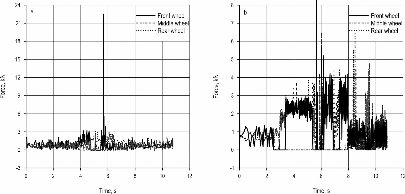
Fig. 15 Force curves for wheels
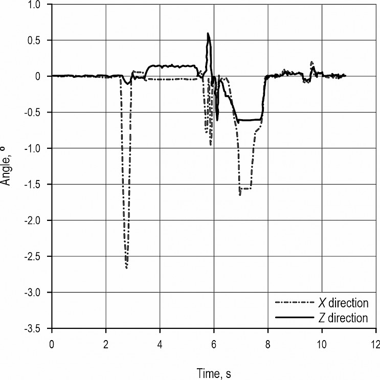
Fig. 16 Frame swing angle during chassis obstacle crossing
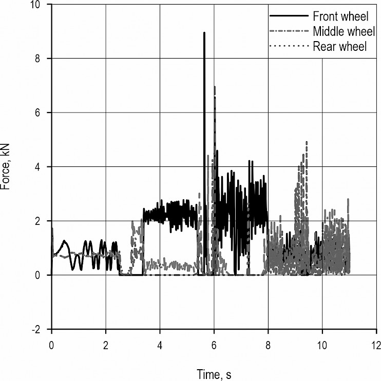
Fig. 17 Wheel force curves
7. Conclusions
Þ Conventional wheeled vehicles have severe mobility limitations in rough terrain. The legged chassis has high degrees of freedom and high control complexity, which limits its mobility in rough terrain. Combining the advantages of a wheeled vehicle and a legged chassis, an SWC&F is proposed as a chassis that drives in rough terrain.
Þ The mathematical model of the chassis structure and the structural calculation formula were established, and the relationship between the rotation angle of the chassis joints and the lifting height of the wheel legs in the process of obstacle crossing was determined. The range of swing angles of each wheel leg is determined according to the installation position of the hydraulic cylinder. Theoretical analysis shows that a maximum crossing height of 411.1 mm can be achieved with an SWC&F.
Þ Using the PID control method and conventional control method, respectively, a joint simulation was performed in ADAMS/Simulink to analyze the barrier-crossing height of the SWC&F. The results show that the chassis virtual prototype using the PID control system can overcome the obstacle with a height of 411 mm in theoretical analysis, and has better dynamic response characteristics, obstacle performance and road adhesion. The optimized chassis has a stronger obstacle surpassing ability and road adhesion in the process of obstacle crossing, which provides a theoretical basis for the design and manufacture of chassis prototypes, and promotes the wheel-legged multi-wheel drive mountain forestry mechanical power chassis. The model fully satisfies the need for the chassis to overcome the obstacles.
Acknowledgements
This work was supported by the Fundamental Research Funds for the Central Universities (Grant No. BJFUKF201822) and Beijing municipal construction project special fund.
8. References
Antonov, A.V., Vorotnikov, S.A., 2017: Solving Kinematic and Dynamic Problems for a Three-Point Wheel-Legged Robot. Proceedings of Higher Educational Institutions. Machine Building (3): 4–11.
Couceiro, M.S., Portugal, D., 2018: Swarming in forestry environments: collective exploration and network deployment. Swarm Intell. Princ. Curr. Algoritm. Methods 119(1): 323–344.
Cristofori, D., Vacca, A., 2012: The Modeling of Electrohydraulic Proportional Valves. Journal of Dynamic Systems Measurement and Control-Transactions of the Asme 134(2): 13 p. https://doi.org/10.1115/1.4005362
Gao, Y.Y., Kang, F., Kan, J.M., Wang, Y.T., Tong, S.Y., 2021: Analysis and Experiment of Cutting Mechanical Parameters for Caragana korshinskii (C.k.) Branches. Forests 12(10): 24 p. https://doi.org/10.3390/f12101359
Kormanek, M., Dvorak, J., 2021: Ground Pressure Changes Caused by MHT 8002HV Crawler Harvester Chassis. Croat. j. for. eng. 42(2): 201–211. https://doi.org/10.5552/crojfe.2021.844
Li, W.H., Kang, F., 2020: Design and Analysis of Steering and Lifting Mechanisms for Forestry Vehicle Chassis. Mathematical Problems in Engineering 2020: Article ID 5971746. https://doi.org/10.1155/2020/5971746
Li, Z.L., Liu, J.H., Sun, Z.B., Yu, C.Z., 2019: Dynamic research and analysis for a wheel-legged harvester chassis during tilting process. Advances in Mechanical Engineering 11(6): 1687814019855453. https://doi.org/10.1177/1687814019855453
McConnell, T.E., 2021: Economic Depreciation of In-Woods Forestry Equipment in the US South. Forest Science 67(2): 135–144. https://doi.org/10.1093/forsci/fxaa044
Oliveira-Nascimento, K.A., Higuchi, N., DeArmond, D., Robert, R.C.G., Arce, J.E., Carvalho, J.P.F., 2021: Environmental Thermal Conditions Related to Performance, Dynamics and Safety of Logging in the Brazilian Amazon. Croat. j. for. eng. 42(3): 419–435. https://doi.org/10.5552/crojfe.2021.865
Qu, J.H., Teeple, C.B., Oldham, K.R., 2017: Modeling Legged Microrobot Locomotion Based on Contact Dynamics and Vibration in Multiple Modes and Axes. Journal of Vibration and Acoustics-Transactions of the Asme 139(3): 031013. https://doi.org/10.1115/1.4035959
Routa, J., Nuutinen, Y., Antti, A., 2020: Productivity in Mechanizing Early Tending in Spruce Seedling Stands. Croat. j. for. eng. 41(1): 1–11. https://doi.org/10.5552/crojfe.2020.619
Sampietro, J.A., de Vargas, D.A., Souza, F.L., Nicoletti, M.F., Bonazza, M., Topanotti, L.R., 2022: Comparison of Forwarder Productivity and Optimal Road Density in Thinning and Clearcutting of Pine Plantation in Southern Brazil. Croat. j. for. eng. 43(1): 65–77. https://doi.org/10.5552/crojfe.2022.1147
Sun, S.F., Wu, J.F., Ren, C.L., Tang, H.L., Chen, J.W., Ma, W.L., Chu, J.W., 2021: Chassis trafficability simulation and experiment of a LY1352JP forest tracked vehicle. Journal of Forestry Research 32(3): 1315–1325. https://doi.org/10.1007/s11676-019-01095-5
Sun, W.C., Li, S.G., Wang, W.Q., Zhao, P.J., Yang, R.Q., 2020: Design of Chassis and Kinematics Research of Wheeled Robot. 4th IEEE Information Technology, Networking, Electronic and Automation Control Conference (ITNEC), Electr Network, Jun 12–14.
Sun, Y.X., Xu, L.Z., Jing, B., Chai, X.Y., Li, Y.M., 2020: Development of a four-point adjustable lifting crawler chassis and experiments in a combine harvester. Computers and Electronics in Agriculture 173: 105416. https://doi.org/10.1016/j.compag.2020.105416
Sun, Z.B., Zhang, D., Li, Z.L., Shi, Y., Wang, N., 2022: Optimum Design and Trafficability Analysis for an Articulated Wheel-Legged Forestry Chassis. Journal of Mechanical Design 144(1): 013301. https://doi.org/10.1115/1.4051539
Thomas, A.T., Parameshwaran, R., Sathiyavathi, S., Starbino, A.V., 2019: Improved Position Tracking Performance of Electro Hydraulic Actuator Using PID and Sliding Mode Controller. Iete Journal of Research 68(3): 1683–1695. https://doi.org/10.1080/03772063.2019.1664341
Wu, H.F., Jia, T.Y., Li, N., Wu, J., Yan, L., 2017: Study on the control algorithm for lower limb exoskeleton based on ADAMS/Simulink co-simulation. Journal of Vibroengineering 19(4): 2976–2986. https://doi.org/10.21595/jve.2017.17303
Yadav, A.K., Gaur, P., 2016: Improved Self-Tuning Fuzzy Proportional-Integral-Derivative Versus Fuzzy-Adaptive Proportional-Integral-Derivative for Speed Control of Nonlinear Hybrid Electric Vehicles. Journal of Computational and Nonlinear Dynamics 11(6): 061013. https://doi.org/10.1115/1.4033685
Zemanek, T., Neruda, J., 2021: Impact on the Operation of a Forwarder with the Wheeled, Tracked-Wheel or Tracked Chassis on the Soil Surface. Forests 12(3): 336. https://doi.org/10.3390/f12030336
Zhou, H.B., Chen, R., Zhou, S., Liu, Z.Z., 2019: Design and Analysis of a Drive System for a Series Manipulator Based on Orthogonal-Fuzzy PID Control. Electronics 8(9): 1051. https://doi.org/10.3390/electronics8091051
Zhu, Y., Kan, J.M., Li, W.B., Kang, F., 2018: A novel forestry chassis with an articulated body with 3 degrees of freedom and installed luffing wheel-legs. Advances in Mechanical Engineering 10(1): 1687814017747101. https://doi.org/10.1177/1687814017747101
Zhu, Y., Kan, J.M., 2016: The design of forestry chassis with articulated body of three degrees of freedom and analysis of its obstacle surpassing ability. Journal of Beijing Forestry University 38(5): 126–132. https://doi.org/ 10.13332/j.1000-1522.20150304
© 2022 by the authors. Submitted for possible open access publication under the
terms and conditions of the Creative Commons Attribution (CC BY) license (http://creativecommons.org/licenses/by/4.0/).
Authors' addresses:
Yaoyao Gao, PhD
e-mail: gaoyy@bjfu.edu.cn
Zechen Zeng
e-mail: 494863869@qq.com
Prof. JiangMing Kan, PhD *
e-mail: kanjm@bjfu.edu.cn
Beijing Forestry University
School of Technology
Beijing 100083
CHINA
* Corresponding author
Received: January 05, 2021
Accepted: May 05, 2022
Original scientific paper