LiDAR Scan Density and Spatial Resolution Effects on Vegetation Fuel Type Mapping

This article presents the performance of a vegetation fuel type (FT) classification based on conditional rules according to the Prometheus system, including an analysis of the effect of cell size and scan density on mapping vertical structural types, exemplified as FT, using exclusively LiDAR data. Since the Prometheus system does not specify any criterion for the minimum extension where those methodologies can be applied, we searched for the optimal classification cell size by gridding the study area at 20 and 40 m cell sizes. We also included a study of the effects of varying the scan density from 2 to 0.5 pulses·m-2. To validate the classification method, we used a stratified random sampling without replacement of 15 cells per FT and made an independent visual assessment of FTs. The best results in terms of precision were obtained for the combination of 0.5 pulses·m-2 and 20 m-resolution dataset, with an overall accuracy of 84.13%. It was also showed that an increase in scan density would not improve the global accuracy of the classification, but it would be desirable for a better detection of the shrub stratum.

LiDAR Scan Density and Spatial Resolution Effects on Vegetation Fuel Type Mapping

Alba García-Cimarras, José Antonio Manzanera, Rubén Valbuena

Abstract

This article presents the performance of a vegetation fuel type (FT) classification based on conditional rules according to the Prometheus system, including an analysis of the effect of cell size and scan density on mapping vertical structural types, exemplified as FT, using exclusively LiDAR data. Since the Prometheus system does not specify any criterion for the minimum extension where those methodologies can be applied, we searched for the optimal classification cell size by gridding the study area at 20 and 40 m cell sizes. We also included a study of the effects of varying the scan density from 2 to 0.5 pulses·m-2. To validate the classification method, we used a stratified random sampling without replacement of 15 cells per FT and made an independent visual assessment of FTs. The best results in terms of precision were obtained for the combination of 0.5 pulses·m-2 and 20 m-resolution dataset, with an overall accuracy of 84.13%. It was also showed that an increase in scan density would not improve the global accuracy of the classification, but it would be desirable for a better detection of the shrub stratum.

Keywords: spatial resolution, scan density, fuel type, prometheus classification system, LiDAR

1. Introduction

The Mediterranean region is frequently affected by wildland fires, consuming thousands of hectares of vegetation and having severe consequences both in the ecosystems and landscape (De Luís et al. 2001, González-Olabarria et al. 2005). Since natural factors influencing wildland fire spread such as topography and meteorology cannot be modified, forest fires may only be prevented by detecting the forest fuel and anticipating potential areas with vertical continuity in the vegetation structure, where the rate of spread, intensity and severity of forest fires are higher (Anderson 1982, Hermosilla et al. 2014). For this purpose, satellite and aerial imagery are not useful by themselves unless combined with active sensors that can retrieve vertical information (especially understory information), such as Light Detection and Ranging (LiDAR), a reliable sensor to analyse forest structure (Bottalico et al. 2017, Valbuena et al. 2013). At landscape scale, the knowledge of forest vertical structure, or its equivalent concept of forest fuel type (FT), is essential. These FTs are groups of vertical vegetation profiles with similar fire behaviour, which according to the Prometheus system (Prometheus S.V. Project. 1999) can be classified in seven different types (Table 1). This system was specifically designed for the Mediterranean region and it is based on the Northern Forest Fire Laboratory (NFFL) classification. The use of LiDAR along with multispectral imagery such as ASTER (Falkowski et al. 2004), Landsat (Skowronski et al. 2007, Marino et al. 2016), QuickBird (Mutlu et al. 2008), Sentinel 2 (Domingo et al. 2020, Sánchez Sánchez et al. 2018, Ruiz et al. 2018) or colour infrared imagery (Jakubowski et al. 2013) among others, to map FT has already been studied. However, despite being an accurate tool, little research has been carried out using exclusively LiDAR data in order to map FT or forest structure (Zimble et al. 2003, Falkowski et al. 2009, van Ewijk et al. 2011, Huesca et al. 2019, Ferrer Palomino and Silva 2021, García-Cimarras et al. 2020).

Table 1 Description of different fuel types (FTs) according to Prometheus classification

It should be noted that FT classifications, including the Prometheus system, do not specify any criterion for the minimum area or cell size where those methodologies can be applied. There is a wide range of possible cell sizes that can be used to estimate forest variables, ranging from fine to coarse scales. Too small cells may lose LiDAR information from the understory, and the map will be too fragmented with a »salt and pepper« effect. Conversely, a too large cell size will classify an excessively broad area, resulting in a coarse, inaccurate classification. Also, the selection of cell size could depend on the density of LiDAR data. Therefore, it is vital to find a balance between these two extremes and choose a cell size that meets wildland fire managers and scientists needs, since it could affect the results of the analysis (Wiens 1989).

Similarly, other studies have focused on studying the effect of LiDAR scan density on the estimation of forest variables (González-Ferreiro et al. 2012, Magnusson et al. 2007, Ruiz et al., 2014, Watt et al. 2013), on predicting characteristics of individual trees (Vauhkonen et al. 2008), or on crown fuel modelling (Marino et al. 2019). However, no research has been carried out with the aim of studying the influence of LiDAR scan density on FT mapping. Therefore, it is necessary to define a minimum threshold of scan density. Otherwise, the information will be insufficient to impute a FT to each cell. Another reason to warrant enough scan density is the need for characterising the shrub stratum. Shrub height is a critical parameter used in the Prometheus classification system to discriminate between forest without understory (FT5), forest with shrubs (FT6) and forest with vertical FT7) (Table 1).

Therefore, the aim of this research is to propose a FT classification and to analyse both the effect of cell size and scan density on mapping vertical structural types, exemplified as FT, by means of LiDAR data.

2. Materials and Methods

2.1 Study Area

The study area was a 2x2 km tile located in La Rioja province (Spain; Fig. 1). We chose this area for our study, in view of its apparent diversity of vegetation structure types.

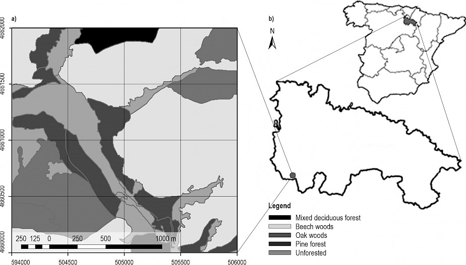
Fig. 1 a) Orthophoto of the study area (2017) with vegetation covers from the Spanish National Forest Map at 25 m scale. Universal Transverse Mercator (UTM) coordinates (m) in the margins; b) Location map of the study area. La Rioja province is shadowed in grey. The study area is the red square

La Rioja has a unique location, affected by both Mediterranean and Atlantic areas of influence, where we can find beech, pine and meso-xerophilous oak forests, among other species (Iñigo et al. 2011). Fig. 1 shows the forest covers of our area of interest that includes forests with the most representative species being Quercus ilex ssp. ballota, Quercus pyrenaica, Quercus petraea, Fagus sylvatica and Pinus sylvestris.

2.2 Lidar Data Acquisition and Processing

The LAZ file corresponding to our study area was downloaded from the Spanish Geographic Institute’s website (Instituto Geografico Nacional 2016). The area has been covered between August and September 2016, therefore, under leaf-on conditions and has 2 pulses·m-2 mean scan density. The 2x2 km file was provided in ETRS89 Datum. The projection was the Universal Transverse Mercator (UTM) Zone 30N, and the coordinates of the upper-left corner were X: 504.000 m; Y: 4.662.000 m.

To study the effect of the cell size on the FT classification, we compared two different cell sizes: 20 and 40 m. The minimum cell size was set to 20 m to ensure at least 200 returns for the analysis with the lower scan density of 0.5 pulses·m-2.

To process the data, an R code (R Core Development Team 2018) was developed using FUSION software v4.10 (McGaughey 2020), as described in Fig. 2. First, the LAZ file was decompressed into a LAS file. Then, the point cloud was filtered with FilteData to remove outliers. Given that the scan density was irregular within the area of interest, the point cloud was previously homogenised to 2 and 0.5 pulses·m-2 using the lidR package in R. Afterwards, ClipData tool extracted the ground pulses from the original point cloud, and after that, GridSurfaceCreate tool used those ground pulses to create a digital terrain model (DTM) at 5x5 m spatial resolution. ClipData tool was used again to subtract the DTM from the original point clouds in order to normalise the point heights and to clip the 10,000 and 2,500 cells for the 20 and 40 m cell sizes, respectively. Finally, Gridmetrics program was used both for 20 and 40 m cell sizes to calculate the LiDAR metrics in the following stratums: from 0.00 to 0.30 m; from 0.30 to 0.60 m; from 0.60 to 2.00 m; from 2.00 to 4.00 m and above 4.00 m, coinciding with the stratums of the Prometheus classification system. Additionally, the forest canopy cover was estimated from the percentage of first returns above 4.00 m.

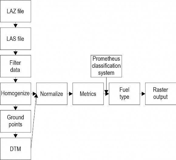
Fig. 2 Flowchart for LiDAR data processing and application of Prometheus classification system

2.3 Fuel Type Classification and Mapping

A FT was assigned to each cell based on conditional rules according to Table 2, which summarises the criteria employed to adapt the Prometheus classification system to the LiDAR information previously extracted. First, when more than 60% of the vegetation was lower than 30 cm height, the cell was directly classified as grasslands (FT1). Then, if Tree Cover was lower than 50%, the cell was assigned to grasslands or shrubs (FT1, FT2, FT3 or FT4) depending on the stratum with the highest number of returns (Mode). When the stratum with the greatest number of returns (Mode) was the stratum above 4 m in height, the assigned FT was determined by consulting the second height interval with more returns (2nd Mode). In the case that the Tree Cover was greater than or equal to 50%, a similar procedure was employed to differentiate those FT corresponding to trees without understory (FT5), trees with shrubs (FT6) and forest with vertical continuity (FT7) by looking the Mode, 2nd Mode and 3rd Mode being discriminated under the criterion on whether vertical continuity of plant material would allow ground fires to spread toward tree crowns. It was assumed that when Max.Elev was above 12 m there will not be vertical continuity because shrubs would not reach the crown base height, and thus those areas were classified as trees with shrubs (FT6). On the other hand, when Max. Elev was equal or lower than 12 m, the canopy base height could be low enough to, in some cases, create a vertical continuity. Lastly, when the Mode was at the >4 m stratum and the 2nd Mode at 2–4 m, there was a need to give an additional criterion defining the distance between understory and crowns, which we addressed by looking at the height of the 3rd Mode. Using this set of recursive rules (Table 2), FT maps were created at 20 and 40 m spatial resolution, respectively, with one value of FT assigned to each cell.

Table 2 Classification system proposed to assign a fuel type (FT) to a cell with LiDAR data

2.4 Data Validation

To validate our method, we tested 15 cells (when it was possible) randomly selected for each FT/cell size/scan density combination. There were some exceptions in the case of low shrubs (FT2), for which only 8 cells were available when the pixel size was 20 m and the scan density 2 pulses·m-2 and when the pixel size was 40 m for both densities, that FT could not be identified in our study area. The validation process consisted on contrasting assigned FT by observing the point cloud extracted in a grid of 20x20 m with the FUSION LDV (LiDAR Data Viewer) 3D visualisation environment (McGaughey 2020), which was considered as reference data, against the automatic classification (Table 2).

To assess the accuracy of the classification, we used a confusion matrix along with the overall accuracy, user’s accuracy, producer’s accuracy and Kappa coefficient (Congalton 1991). The results of the confusion matrix were weighted to the proportion of area covered by each FT (Olofsson et al. 2013; Stehman 1996). Eq. 1 was applied to obtain the weighted proportion (pij) of a sample for visually referenced FT j and the automatically classified FT i.

(1)

Where:

Aj/At the ratio between the area (Aj) observed for each FT class j with respect to the total number of cells (At=2500, with a cell size of 40 m, or 10,000, with a cell size of 20 m)

nij the number of cells observed for class j and predicted to be class i, and ni is the total number of plots validated for a class i.

3. Results

When the density was fixed at 0.5 pulses·m-2 and the cell size was set at 40 m (Fig. 3a), the overall accuracy obtained was 79.33% (Table 3). No cells were classified as low shrubs (FT2). The worst results were found when trying to discriminate between trees with shrubs (FT6; producers’ accuracy 0.25) and forest with vertical continuity (FT7; producers’ accuracy 0.65; users’ accuracy 0.40; Table 3).

Table 3 Confusion matrix corresponding to 0.5 pulses·m-2 and pixel size of 40 m

Table 4 displays the confusion matrix obtained for the 0.5 pulses·m-2 dataset with cell size of 20 m (Fig. 3b). The global accuracy was 84.13% (Table 4). In this case, the user’s accuracy obtained when discriminating between trees with shrubs (FT6) and forest with vertical continuity (FT7) was very low (0.40 and 0.20, respectively; Table 4). Producers’ accuracy was low for high shrubs (FT4) and forest with shrubs (FT6), 0.42 and 0.30, respectively (Table 4).

Table 4 Confusion matrix corresponding to 0.5 pulses·m-2 and pixel size of 20 m

When the scan density was increased to 2 pulses·m-2 with a cell size of 40 m (Fig. 3c, Table 5), the global accuracy was 78.83%. However, no cells were classified as low shrubs (FT2). User’s accuracies values were high (from 0.73), but the identification of trees with shrubs (FT6) was less efficient (0.13) than for other FT (0.52 or more, Table 5).

Table 5 Confusion matrix corresponding to 2 pulses·m-2 and pixel size of 40 m

Table 6 shows the confusion matrix obtained for the dataset with a cell size of 20 m and 2 pulses·m-2 (Fig. 3d). The global accuracy was 81.11%. The highest levels of error were found in the discrimination between trees with shrubs (FT6) and forest with vertical continuity (FT7). Since the group low shrubs (FT2) was underrepresented in the study area (only 8 cells out of 10,000), its weighted producer’s accuracy was low even though no samples were classified wrongly. In addition, producer’s accuracy for trees with shrubs (FT6) was the second lowest result due to the low number of cells classified as this FT (162 out of 10,000). The rest of the user’s and producer’s accuracies values were higher (0.54 or greater).

Table 6 Confusion matrix corresponding to dataset with 2 pulses·m-2 and pixel size of 20 m

In summary, we observed that an increase in the scan density from 0.5 to 2 pulses·m-2 did not result in an increase of the overall classification accuracy independently of the pixel size. In addition, the best results in terms of overall accuracy were provided by the 0.5 pulses·m-2 scan density, and 20 m pixel size configuration. Losing spatial resolution would lead to the incapacity of detecting the scarcely represented species such as low shrubs (FT2). On the other hand, the highest scan density (2 pulses·m-2) combined with the smallest cell size (20 m) provided both satisfactory FT classification and spatial resolution. Additionally, a high correspondence between the output raster (Fig. 3) and the orthophoto (Fig. 1) of the study area was observed.

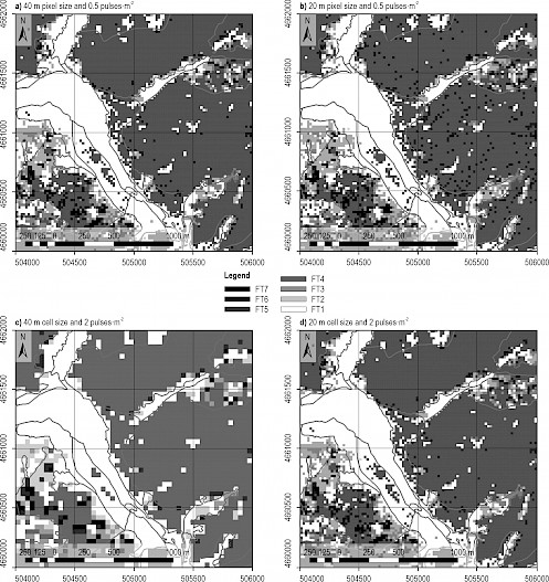
Fig. 3 Output rasters for fuel type (FT) classification datasets. The polygons of the vegetation cover types from the Spanish National Forest Map from Fig. 1 have been superposed as spatial reference. FT1: Grasslands; FT2: Low shrubs; FT3: Medium shrubs; FT4: High shrubs; FT5: Forest without understory; FT6: Forest with shrubs; FT7: Forest with vertical continuity

To validate our classification methodology, the output raster of the study area, gridded using 40 m cell size with a scan density of 0.5 pulses·m-2, was resampled to 20 m cell size and compared with the output raster obtained when the study area was classified with a pixel size of 20 m (Fig. 4a). It was observed that 80.27% of the cells remained classified with the same FT (Table 7), while 11.47% of the cells were classified as an FT of lower vegetation height and 8.26% changed to an FT of taller vegetation.

Table 7 Number of coincidences (in bold) and mismatches during fuel type (FT) classification with 0.5 pulses·m-2 scan density. Gridding of the 40 m cell map was resampled from 40 m to 20 m cell size. Total number of cells: 10,000. Numbers of cells with the same fuel type assignment for both cell sizes are in bold

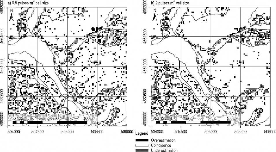
Fig. 4 Changes in fuel type (FT) classification by comparing the classifications with 40 m and 20 m cell size. Overestimation: mismatch in the classification as assignment to a FT of taller vegetation height. Coincidence: match between both classifications; Underestimation: mismatch in the classification as assignment to a FT of lower vegetation height. The polygons of the vegetation cover types from the Spanish National Forest Map from Fig. 1 have been superposed as spatial reference

The same procedure was carried out to compare the 20 and 40 m cell size with 2 pulses·m-2 classification (Fig. 4b). We observed that 84.56% of the cells were classified as the same FT using the two different cell sizes (Table 8), while 6.87% of the cells were classified as an FT of lower vegetation height and 8.57% changed to an FT of taller vegetation.

For both scan densities, 0.5 and 2 pulses·m-2, low shrubs (FT2) were not detected when a cell size of 40 m was used. However, with the 20 m cell size, this FT was detected in spite of its scarce presence in the area (Tables 7 and 8). On the other hand, grasslands (FT1) and forest without understory (FT5) were the most represented FT and the most stable ones in all possible cases.

Table 8 Number of coincidences (in bold) and mismatches during fuel type (FT) classification with 2 pulses·m-2 scan density

4. Discussion

We have assessed the vegetation structure in an area representative of the FT diversity in a Mediterranean mountain vegetation ecosystem, using LiDAR data resampled at 20 m or 40 m cell size with scan densities of 0.5 or 2 pulses·m-2. The presented methodology provides a simple, inexpensive and reliable method that uses open-source data available for the Spanish territory that can be replicable in other areas with public LiDAR coverage, and furthermore, provides a high overall accuracy to map FT according to the Prometheus classification system.

Other authors also aimed to map FTs using LiDAR technology to achieve the distinction between only two different forest structures (Zimble et al. 2003) or only four different stages of forest stand development (van Ewijk et al. 2011), both using a 30 m cell size and obtaining good results (97% and 90%, respectively). Classifications of more diverse types, at least six or seven different FTs, either obtained 55% overall accuracy (Huesca et al. 2019), using a 30 m grid and a LiDAR scan density of 0.5 pulses·m-2, or recurred to elaborated methods such as Random Forest algorithm and expensive private flights to obtain a global accuracy of 95.54% in the case of distinguishing 6 FTs and 90.12% in the case of 7 FTs (Falkowski et al. 2009). That is also the case of Hill and Thomson (2005), who used complex methods including segmentation algorithm, Principal Components Analysis and unsupervised classification, to obtain an overall accuracy of 94% for classifying ten different structurally based vegetation type classes by integrating LiDAR with a scan density of 4.83 pulses·m-2 and hyperspectral data. Similarly, Garcia et al. (2011) used a higher LiDAR scan density (between 1.5 and 6 pulses·m-2) and a 30 m cell size, plus an Airborne Topographic Mapper (ATM) multi-spectral sensor with 11 different bands, to calculate Normalized Difference Vegetation Index (NDVI) and other spectral indices. Their methodology yielded an overall accuracy of 88.24% and had to resample the ATM image from 2 to 6 m pixel size in order to ensure a sufficient number of LiDAR pulses per pixel to retrieve the metrics. Their results were slightly better than those obtained by Riaño et al. (2002), who used Landsat Thematic Mapper ™ images and ancillary data (82.8%), but it should be noted that the methodology they used was far more complex than the one presented in this research.

The methodology proposed in the present study has shown more accurate results than those obtained by Arroyo et al. (2006) with a Quickbird image and ancillary data, whose overall accuracy was 75% with the Kappa coefficient of 0.69, and those of Falkowski et al. (2004), who used ASTER imagery to map FT to obtain an accuracy of 77%.

A conclusion from the results presented in Tables 5 and 6 is that we observed a slight decrease in the overall accuracy when the cell size was reduced from 20 to 40 m at the 2 pulses·m-2 LiDAR density. As a consequence, sparsely represented FTs, such as low shrubs (FT2), were undetectable with the coarser cell size (40 m), but »reappeared« with the finer (20 m) cell size. Therefore, and even though the accuracy to distinguish between trees with shrubs (FT6) and forest with vertical continuity (FT7) was suboptimal, we recommend using the 20 m grid because a better spatial resolution provides a closer representation to reality. Nonetheless, cell size cannot be indefinitely decreased for FT classification purposes, because the well-known »salt and pepper« problem in FT mapping would arise (Arroyo et al. 2006). Therefore, it is vital to choose a cell size in accordance with the research purpose (Woodcock and Strahler 1987) and with the scan density available to ensure a minimum of returns within the cells. For example, Mutlu et al. (2008) used a cell size of 16 m and a point density of 2.58 pulses·m-2, ensuring at least 660 points within a cell, which is enough to map FTs according to our methodology. These authors obtained an overall accuracy of 90% but they also used a far more complex methodology (minimum noise fraction) than ours and their study area was not representative in terms of altitude and slope of a Mediterranean forest.

At a fixed cell size of 20 m, the overall accuracy was 3.02% higher in the case of a LiDAR density of 0.5 pulses·m-2 (Tables 3 and 5). Then, a higher scan density, that is, greater number of returns, did not result in a higher overall accuracy. The overall accuracy was almost identical when the scan density increased from 0.5 to 2 pulses·m-2 and the cell size was 40 m (Tables 4 and 6). However, even though an increase of scan density did not result in an increase of the overall accuracy, it would be desirable when mapping FTs, especially to discriminate between forest FTs (FT5, FT6 and FT7) (García et al. 2011). In addition, van Ewijk et al. (2011) increased the scan density of their LiDAR dataset from 3 to 10 pulses·m-2 by flying the same area twice. Because of the low scan density of our datasets, few returns could penetrate the canopy, especially in the case of dense forests (Lee et al. 2004). Consequently, the information obtained from the shrub stratum was in some cases limited or missing, and thus there were errors in the discrimination between forest FTs (FT5, FT6 and FT7), a shortcoming also noticed by Adnan et al. (2017), García et al. (2011), Riaño et al. (2002) and Evans et al. (2009).

One of the most challenging tasks was to discriminate between forest with shrubs (FT6) and forest with vertical continuity (FT7). The errors committed identifying these FTs were usually because, according to the Prometheus classification system, vegetation below 4 meters is considered shrub. Therefore, if the tree canopies are slightly higher than 4 m, the canopy also covers the interval from 2.00 to 4.00 m. In case the shrub stratum is low, even though the distance between the crown base and the shrub stratum is more than half a meter (FT6), it would be mistakenly classified as forest with vertical continuity (FT7) because the stratum with the largest amount of returns is the interval from 2.00 to 4.00 m. Additionally, in cases where the shrub stratum is high but with no vertical continuity with the tree stratum, which is higher than 4.00 m, the distance between the crown base and the shrub stratum again may be more than 0.5 m and the cell will be classified as forest with vertical continuity (FT7) when it should be forest with shrubs (FT6). Depending on the vegetation height, this could be mitigated by changing the criterion from forest with vertical continuity (FT7) to forest with shrubs (FT6) in the case when the canopy cover is greater than or equal to 50%, the interval with the greater number of returns is the one above 4.00 and the second interval with the greater number of returns is from 2.00 to 4.00 m (Table 2). In this study a forest with vertical continuity (FT7) was chosen in that case because it was more restrictive.

The comparison of the FT classification results between gridding the study area at 40 m and at 20 m can be considered as an indirect method for the validation of the expert classification criterion, with an 80.27% and 84.56% reliability for 0.5 and 2 pulses·m-2, respectively (Tables 7 and 8). This comparison also shows how an increase in the scan density resulted in a more accurate classification. Nevertheless, some cells were wrongly classified due to eventual errors of validation given that sometimes the amount of returns in an interval detected with the naked eye seemed slightly higher or lower. This explains the errors made when trying to discriminate grasslands (FT1) from low shrubs (FT2) or low shrubs (FT2) from medium shrubs (FT3), for instance. In case of doubt, the FT of higher fire risk was selected. Another source of errors was the assessment of the canopy cover, which would explain the error made between grasslands (FT1) and forest without understory (FT5); low shrubs (FT2) and forest with shrubs (FT6); medium shrubs (FT3), high shrubs (FT4) and forest with vertical continuity (FT7).

5. Conclusions

In conclusion, this methodology has proven to be effective for assessing and mapping FTs and we have demonstrated the advantages of using the proper LiDAR scan density and cell grid to map structural vegetation types and FTs. It was observed that an increase in the scan density from 0.5 to 2 pulses·m-2 did not result in an increase of the overall classification accuracy independently of the pixel size. In addition, losing spatial resolution would lead to the incapacity of detecting the scarcely represented FTs. It should be reduced according to the LiDAR scan density to guatantee a minimum number of point per cell and also trying to avoid the salt and pepper effect. Future improvements should consider a better classification criterion to distinguish between forest with shrubs (FT6) and forest with vertical continuity (FT7) and also to estimate the forest cover. The fusion of this LIDAR-based methodology with other sensors, such as spectral imagery, could also be considered in the future.

Acknowledgments

This work was supported by the Ministerio de Educación, Cultura y Deporte under Grant FPU17/00423.

6. References

Adnan, S., Maltamo, M., Coomes, D.A., Valbuena, R., 2017: Effects of Plot Size, Stand Density and Scan Density on the Relationship between Airborne Laser Scanning Metrics and the Gini Coefficient of Tree Size Inequality. Canadian Journal of Forest Research 47(12): 1590–1602. https://doi.org/10.1139/cjfr-2017-0084

Anderson, H.E., 1982: Aids to Determining Fuel Models for Estimating Fire Behavior. USDA Forest Service, Intermountain Forest and Range Experiment Station. General Technical Report INT-122, 22 p.

Arroyo, L.A., Healey, S.P., Cohen, W.B., Cocero, D., Manzanera, J.A., 2006: Using Object-Oriented Classification and High-Resolution Imagery to Map Fuel Types in a Mediterranean Region. Journal of Geophysical Research: Biogeosciences 111(4): 1–10. https://doi.org/10.1029/2005JG000120

Bottalico, F., Chirici, G., Giannini, R., Mele, S., Mura, M., Puxeddu, M., McRoberts, R.E., Valbuena, R., Travaglini, D., 2017: Modeling Mediterranean Forest Structure Using Airborne Laser Scanning Data. International Journal of Applied Earth Observation and Geoinformation 57: 145–153. https://doi.org/10.1016/j.jag.2016.12.013

Congalton, R.G., 1991: A Review of Assessing the Accuracy of Classifications of Remotely Sensed Data. Remote Sensing of Environment 37(1): 35–46. https://doi.org/10.1016/0034-4257(91)90048-B

De Luís, M., García-Cano, M.F., Cortina, J., Raventós, J., González-Hidalgo, J.C., Sánchez, J.R., 2001: Climatic Trends, Disturbances and Short-Term Vegetation Dynamics in a Mediterranean Shrubland. Forest Ecology and Management 147(1): 25–37. https://doi.org/10.1016/S0378-1127(00)00438-2

Domingo, D., de la Riva, J., Lamelas, M.T., García-Martín, A., Ibarra, P., Echeverría, M., Hoffrén, R., 2020: Fuel Type Classification Using Airborne Laser Scanning and Sentinel 2 Data in Mediterranean Forest Affected by Wildfires. Remote Sensing12(21): 3660. https://doi.org/10.3390/rs12213660

Evans, J.S., Hudak, A.T., Faux, R., Smith, A.M.S., 2009: Discrete Return Lidar in Natural Resources: Recommendations for Project Planning, Data Processing, and Deliverables. Remote Sensing 1(4): 776–794. https://doi.org/10.3390/rs1040776

Falkowski, M.J., Evans, J.S., Martinuzzi, S., Gessler, P.E., Hudak., A.T., 2009: Characterizing Forest Succession with Lidar Data: An Evaluation for the Inland Northwest, USA. Remote Sensing of Environment 113(5): 946–956. https://doi.org/10.1016/j.rse.2009.01.003

Falkowski, M.J, Gessler, P., Morgan, P., Smith, A.M.S., Hudak, A.T., 2004: Evaluating ASTER Satellite Imagery and Gradient Modeling for Mapping and Characterizing Wildland Fire Fuels. In ASPRS Annual Conference Proceedings. Denver, Colorado.

Ferrer Palomino, A., Silva, F.R.y., 2021: Fuel Modelling Characterisation Using Low-Density LiDAR in the Mediterranean: An Application to a Natural Protected Area. Forests12(8): 1011. https://doi.org/10.3390/f1208101

García-Cimarras, A., Manzanera, J.A., Valbuena, R., 2021: Analysis of Mediterranean Vegetation Fuel Type Changes Using Multitemporal LiDAR. Forests12(3): 335. https://doi.org/10.3390/f12030335

González-Ferreiro, E., Diéguez-Aranda, U., Miranda, D., 2012: Estimation of Stand Variables in Pinus Radiata D. Don Plantations Using Different LiDAR Pulse Densities. Forestry 85(2): 281–292. https://doi.org/10.1093/forestry/cps002

González-Olabarria, J.R., Palahí, M., Pukkala. P., 2005: Integrating Fire Risk Considerations in Forest Management Planning in Spain – A Landscape Level Perspective. Landscape Ecology 20(8): 957–970. https://doi.org/10.1007/s10980-005-5388-8

Hermosilla, T., Ruiz, L.A., Kazakova, A.N., Coops, N.C., Moskal, L.M., 2014: Estimation of Forest Structure and Canopy Fuel Parameters from Small-Footprint Full-Waveform LiDAR Data. International Journal of Wildland Fire 23(2): 224–233. https://doi.org/10.1071/WF13086

Hill, R.A., Thomson, A.G., 2005: Mapping Woodland Species Composition and Structure Using Airborne Spectral and LIDAR Data. International Journal of Remote Sensing 26(17): 3763−3779. https://doi.org/10.1080/01431160500114706

Huesca, M., Riaño, D., Ustin, S.L., 2019: Spectral Mapping Methods Applied to LiDAR Data: Application to Fuel Type Mapping. International Journal of Applied Earth Observation and Geoinformation 74: 159–168. https://doi.org/10.1016/j.jag.2018.08.020

Iñigo, V., Andrades, M., Alonso-Martirena, J.I., Marín, A., Jiménez-Ballesta, R., 2011: Multivariate Statistical and GIS-Based Approach for the Identification of Mn and Ni Concentrations and Spatial Variability in Soils of a Humid Mediterranean Environment: La Rioja, Spain. Water, Air, and Soil Pollution 222(1): 271–284. https://doi.org/10.1007/s11270-011-0822-9

Instituto Geografico Nacional, 2016: IGN. http://centrodedescargas.cnig.es/CentroDescargas/index.jsp

Jakubowski, M.K., Guo, Q., Collins, B., Stephens, S., Kelly, M., 2013: Predicting Surface Fuel Models and Fuel Metrics Using Lidar and CIR Imagery in a Dense, Mountainous Forest. Photogrammetric Engineering & Remote Sensing 79(1): 37–49. https://doi.org/10.14358/PERS.79.1.37

Lee, A., Lucas, R., Brack, C., 2004: Quantifying Vertical Forest Stand Structure Using Small Footprint Lidar to Assess Potential Stand Dynamics. International Archives of Photogrammetry, Remote Sensing and Spatial Information Sciences 34(30): 213–217.

Magnusson, M., Fransson, J.E.S., Holmgren, J., 2007: Effects on Estimation Accuracy of Forest Variables Using Different Pulse Density of Laser Data. Forest Science 53(6): 619–626. https://doi.org/10.1093/forestscience/53.6.619

Marino, E., Ranz, P., Tomé, J.L., Noriega, M.A., Esteban, J., Madrigal, J., 2016: Generation of High-Resolution Fuel Model Maps from Discrete Airborne Laser Scanner and Landsat-8 OLI: A Low-Cost and Highly Updated Methodology for Large Areas. Remote Sensing of Environment 187: 267–280. https://doi.org/10.1016/j.rse.2016.10.020

Marino, E., Tomé, J.L., Madrigal, J., Hernando, C., 2019: Effect of Airborne LiDAR Pulse Density on Crown Fuel Modelling. In Proceedings for the 6th International Fire Behavior and Fuels Conference, 1–6. Marseille, France: International Association of Wildland Fire.

McGaughey, R.J., 2020: FUSION/LDV: Software for LIDAR Data Analysis and Visualization, no. August.

Mutlu, M., Popescu, S.C., Stripling, C., Spencer, T., 2008: Mapping Surface Fuel Models Using Lidar and Multispectral Data Fusion for Fire Behavior. Remote Sensing of Environment 112(1): 274–285. https://doi.org/10.1016/j.rse.2007.05.005

Olofsson, P., Foody, G.M., Stehman, S.V., Woodcock, C.E., 2013: Making Better Use of Accuracy Data in Land Change Studies: Estimating Accuracy and Area and Quantifying Uncertainty Using Stratified Estimation. Remote Sensing of Environment 129: 122–131. https://doi.org/10.1016/j.rse.2012.10.031

Prometheus S.V. Project, 1999: Management Techniques for Optimisation of Suppression and Minimization of Wildfire Effect. European Commission – Contract Number ENV4-CT98-0716.

R Core Development Team, 2018: R: A Language and Environment for Statistical. Vienna, Austria. https://doi.org/10.1007/978-3-540-74686-7

Riaño, D., Chuvieco, E., Salas, J., Palacios-Orueta, A., Bastarrika, A., 2002: Generation of Fuel Type Maps from Landsat TM Images and Ancillary Data in Mediterranean Ecosystems. Canadian Journal of Forest Research 32(8): 1301–1315. https://doi.org/10.1139/x02-052

Ruiz, L.A., Recio, J.A., Crespo-Peremarch, P., Sapena, M., 2018: An object-based approach for mapping forest structural types based on low-density LiDAR and multispectral imagery. Geocarto International 33(5): 443–457. https://doi.org/10.1080/10106049.2016.1265595

Ruiz, L.A., Hermosilla, T., Mauro, F., Godino, M., 2014: Analysis of the Influence of Plot Size and LiDAR Density on Forest Structure Attribute Estimates. Forests 5(5): 936–951. https://doi.org/10.3390/f5050936

Sánchez Sánchez, Y., Martínez-Graña, A., Santos Francés, F., Mateos Picado, M., 2018: Mapping Wildfire Ignition Probability Using Sentinel 2 and LiDAR (Jerte Valley, Cáceres, Spain). Sensors 18(3): 826. https://doi.org/10.3390/s18030826

Skowronski, N., Clark, K., Nelson, R., Hom, J., Patterson, M., 2007: Remotely Sensed Measurements of Forest Structure and Fuel Loads in the Pinelands of New Jersey. Remote Sensing of Environment 108(2): 123–129. https://doi.org/10.1016/j.rse.2006.09.032

Stehman, S.V., 1996: Estimating the Kappa Coefficient and Its Variance under Stratified Random Sampling. Photogrammetric Engineering and Remote Sensing 62(4): 401–407

Valbuena, R., Maltamo, M., Martín-Fernández, S., Packalen, P., Pascual, C., Nabuurs, G-J., 2013: Patterns of Covariance between Airborne Laser Scanning Metrics and Lorenz Curve Descriptors of Tree Size Inequality. Canadian Journal of Remote Sensing 39(sup1): S18–S31. https://doi.org/10.5589/m13-012

van Ewijk, K.Y., Treitz, P.M., Scott, N.A., 2011: Characterizing Forest Succession in Central Ontario Using Lidar-Derived Indices. Photogrammetric Engineering and Remote Sensing 77(3): 261–269. https://doi.org/10.14358/PERS.77.3.261

Vauhkonen, J., Tokola, T., Maltamo, M., Packalén, P., 2008: Effects of Pulse Density on Predicting Characteristics of Individual Trees of Scandinavian Commercial Species Using Alpha Shape Metrics Based on Airborne Laser Scanning Data. Canadian Journal of Remote Sensing 34(sup2): S441–S459. https://doi.org/10.5589/m08-052

Watt, M.S., Adams, T., Gonzalez Aracil, S., Marshall, H., Watt, P., 2013: The Influence of LiDAR Pulse Density and Plot Size on the Accuracy of New Zealand Plantation Stand Volume Equations. New Zealand Journal of Forestry Science 43(1): 15. https://doi.org/10.1186/1179-5395-43-15

Wiens, J.A., 1989: Spatial Scaling in Ecology. Functional Ecology 3(4): 385–397. https://doi.org/10.2307/2389612

Woodcock, C.E., Strahler, A.H, 1987: The Factor of Scale in Remote Sensing. Remote Sensing of Environment 21(3): 311–332. https://doi.org/10.1016/0034-4257(87)90015-0

Zimble, D.A., Evans, D.L., Carlson, G.C., Parker, R.C., Grado, S.C., Gerard, P.D., 2003: Characterizing Vertical Forest Structure Using Small-Footprint Airborne LiDAR. Remote Sensing of Environment 87(2–3): 171–182. https://doi.org/10.1016/S0034-4257(03)00139-1

© 2022 by the authors. Submitted for possible open access publication under the
terms and conditions of the Creative Commons Attribution (CC BY) license (http://creativecommons.org/licenses/by/4.0/).

Authors' addresses:

Alba García-Cimarras, MSc *

e-mail: alba.gcimarras@upm.es

Prof. José Antonio Manzanera, PhD

e-mail: joseantonio.manzanera@upm.es

Universidad Politécnica de Madrid

Escuela de Montes, Forestal y del Medio Natural

Calle José Antonio Novais 10

28040, Madrid

SPAIN

Prof. Rubén Valbuena, PhD

e-mail: r.valbuena@bangor.ac.uk

Bangor University

School of Natural Sciences

Bangor University. Thoday building

LL57 2UW Bangor

UK

* Corresponding author

Received: May 01, 2021

Accepted: July 30, 2022

Original scientific paper