A review of Sensors, Sensor-Platforms and Methods Used in 3D Modelling of Soil Displacement after Timber Harvesting

Proximal sensing technologies are becoming widely used across a range of applications in environmental sciences. One of these applications is in the measurement of the ground surface in describing soil displacement impacts from wheeled and tracked machinery in the forest. Within a period of 2–3 years, the use photogrammetry, LiDAR, ultrasound and time-of-flight imaging based methods have been demonstrated in both experimental and operational settings. This review provides insight into the aims, sampling design, data capture and processing, and outcomes of papers dealing specifically with proximal sensing of soil displacement resulting from timber harvesting. The work reviewed includes examples of sensors mounted on tripods and rigs, on personal platforms including handheld and backpack mounted, on mobile platforms constituted by forwarders and skidders, as well as on unmanned aerial vehicles (UAVs). The review further highlights and discusses the benefits, challenges, and some of the shortcomings of the various technologies and their application as interpreted by the authors.

The majority of the work reviewed reflects pioneering approaches and innovative applications of the technologies. The studies have been carried out almost simultaneously, building on little or no common experience, and the evolution of standardized methods is not yet fully apparent. Some of the issues that will likely need to be addressed in developing this field are (i) the tendency toward generating apparently excessively high resolution micro-topography models without demonstrating the need for or contribution of such resolutions on accuracy, (ii) the inadequacy of conventional manual measurements in verifying the accuracy of these methods at such high resolutions, and (iii) the lack of a common protocol for planning, carrying out, and reporting this type of study.

A review of Sensors, Sensor-Platforms and Methods Used in 3D Modelling of Soil Displacement after Timber Harvesting

Bruce Talbot, Rasmus Astrup

Abstract

Proximal sensing technologies are becoming widely used across a range of applications in environmental sciences. One of these applications is in the measurement of the ground surface in describing soil displacement impacts from wheeled and tracked machinery in the forest. Within a period of 2–3 years, the use photogrammetry, LiDAR, ultrasound and time-of-flight imaging based methods have been demonstrated in both experimental and operational settings. This review provides insight into the aims, sampling design, data capture and processing, and outcomes of papers dealing specifically with proximal sensing of soil displacement resulting from timber harvesting. The work reviewed includes examples of sensors mounted on tripods and rigs, on personal platforms including handheld and backpack mounted, on mobile platforms constituted by forwarders and skidders, as well as on unmanned aerial vehicles (UAVs). The review further highlights and discusses the benefits, challenges, and some of the shortcomings of the various technologies and their application as interpreted by the authors.

The majority of the work reviewed reflects pioneering approaches and innovative applications of the technologies. The studies have been carried out almost simultaneously, building on little or no common experience, and the evolution of standardized methods is not yet fully apparent. Some of the issues that will likely need to be addressed in developing this field are (i) the tendency toward generating apparently excessively high resolution micro-topography models without demonstrating the need for or contribution of such resolutions on accuracy, (ii) the inadequacy of conventional manual measurements in verifying the accuracy of these methods at such high resolutions, and (iii) the lack of a common protocol for planning, carrying out, and reporting this type of study.

Keywords: proximal sensing, post-harvest, site impact, wheel rutting, TLS, photogrammetry

1. Introduction

Following forest operations, wheel rutting and soil displacement provide some of the most obvious traces of forest machine traffic and are commonly used as a proxy for quantifying the environmental impact of an operation on the forest floor (Cambi et al. 2015, Cudzik et al. 2017). In recent years, there has been a resurgence of work addressing the measurement of site disturbance in line with a strategic focus on adaption to climate change, with expected longer periods of lower soil bearing capacity, as well as in increased public concern over the effect of forest operations on soil and the environment in general. The environmental impact on the soil due to forest operations can be considered as a function of the severity of soil displacement, the extent of the displacement on a spatial scale, and the consequences of the impact, e.g. waterlogging due to irreversible compaction (Fig. 1).

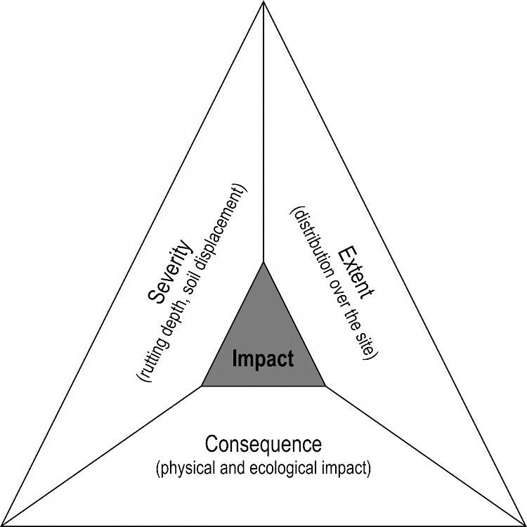
Fig. 1 Overall site soil impact seen as a function of disturbance severity, extent of disturbance over the site, and consequence of disturbance

The manual measurement of wheel rutting and soil displacement on a harvesting site is known to be resource demanding. Thus, the actual sampling intensities used in both research and operations settings are normally low and have been shown to be associated with large sample error at a site level that can call into question the overall validity of carrying out the site impact survey at all (Talbot et al. 2017b).

Advances in sensor technologies offer significant opportunities in simplifying data capture in forest operations in general, and specifically so for measuring large and difficult to quantify effects, such as the extent and severity of soil displacement (Talbot et al. 2017a). In recent years, researchers have proposed several approaches for measuring soil impacts with a focus on both the extent and severity of soil displacement. The main objective of this review is to provide an overview and a broad mutual comparison of these new technologies and their areas of application. This is done to allow an assessment of their apparent suitability for use in research trials and potential future use in an operational forestry setting to be made. All the work considered in this review is categorized as proximal sensing (Mulla 2013), but also includes sensors on UAVs as it remains close-range in comparison with other aerial or even space-borne remote sensing platforms used in forestry. Common for all technologies considered is that they provide a continuous transect or surface model in representing soil displacement, such as in the case of wheel rutting. Further, the digital terrain models (DTMs) described in this review have point resolutions typically tens to hundreds-of-thousands of times higher than the aggregated 1x1 m digital terrain models currently available from ALS data. While the proximal sensing methods discussed here primarily measure the severity, the review also attempts to categorize the contributions of the reviewed papers in terms of their potential in addressing the overall topic of site impact.

The aim of this review is thus to provide an overview of the technologies and methods that have been developed in mapping soil displacement and to provide an evaluation of these in terms of their suitability as research or operational tools in assessing soil displacement arising from forest operations. The review is structured in four main sections:

Þ an overview of the different sensor technologies

Þ the actual settings in which the technologies were applied or considered

Þ the data capture platforms that were deployed

Þ data processing methods, model resolution, and determination of soil displacement is discussed.

2. Overview of sensor technologies used in modelling soil displacement

This section provides a brief introduction to the technologies and methods that have been demonstrated in modelling soil displacement in relation to soil displacement following forest operations.

2.1 Photogrammetry

Photogrammetry involves estimating the three-dimensional coordinates of points on a surface using measurements made in one or more photographic images. Three-dimensional modelling with monocular camera is enabled by Structure-from-Motion (SfM), where images are captured from a number of different positions and matched in an overlay that enables depth perception. In recent years, SfM has been applied in the analysis of a number of forestry problems ranging from forest inventory to forest operations (Iglhaut et al. 2019). The accuracy of photogrammetric models is determined by the clarity and resolution of the images, as well as the existence of sufficient overlap between successive images (typically 70–80%). The surface texture of the object being modelled plays an important role in photogrammetry, and stationary water constitutes a problem for the method, often resulting in no data representation on such surfaces. With 8 studies reported here, photogrammetry is currently the predominant method of 3D modelling of forest machine induced soil displacement in the literature. Close-range photogrammetry from consumer-grade cameras can provide point clouds with multiple millions of points per m2.

2.2 LiDAR

LiDAR (Light Detection and Ranging) is a robust measuring technology that can penetrate sparse vegetation, works independently of light conditions and is well established for both operational and research use in forest inventory and mapping, e.g. Kangas et al. (2018). Basically, the LiDAR system measures the distance between an object and sensor and includes both technology that relies on a beam emitter and rotating mirrors that steer the beam, while new developments include solid state LiDARs that have no moving parts and simultaneously evaluate a number of beams (e.g. Leddar Pixell). The sampling rates, effective ranges and footprints of the various LiDAR systems vary considerably between models (Table 1). Four LiDAR based papers are included in the review.

2.3 Ultrasound

Similar to the case for light in LiDAR, ultrasonic sensors emit and record travel times for ultrasonic waves, however ultrasonic sensors use a single oscillator to emit and receive waves alternately. The sensors seen in this review use only a single source producing 1-dimensional data (point data) when static. While noise pollution in the same frequency can affect the quality of the measurements, ultrasonic waves do reflect off transparent surfaces, meaning that water depth in a rut could be determined, and signal detection is not strongly affected by dust or dirt. Ultrasonic sensors are also generally available at considerably lower cost than optical sensors. The two papers reviewed demonstrate their versatility in two quite different settings.

2.4 Depth cameras

While LiDAR is considered a time-of-flight camera, being based on the time taken for a transmitted signal to return to the sensor, the depth cameras referred to as such in this paper are the devices developed to detect motion and depth for interacting with a gaming console, such as Microsoft’s Kinect® camera developed for the Xbox. These cameras integrate a colour camera sensor (RGB) and an infrared sensor producing both greyscale and depth images, where the sensing range is adjustable (Melander and Ritala 2018). Interestingly, the two papers reviewed here apply the original Kinect and Kinect V2, respectively, where the latter includes some important developments making it more suitable for outside application.

3. Sensor application purpose and setting

The application of new sensor technologies for characterizing soil displacement can be broadly categorized into three categories as either having the aim of:

Þ proof-of-concept for the technology, i.e. demonstrating that the method provides a reliable model of micro-topography

Þ applying the technology to describe differences in machine and wheel configurations on the soil displacement

Þ actually monitoring soil displacement in an operational environment (Table 2).

The measurement technologies have been applied in a range of settings and for different purposes. The applications can be static or mobile, terrestrial or airborne, and used in real-time or post-operations analysis. Applications in a controlled environment have either sought to demonstrate the measurement technology itself (proof-of-concept), or to document at a level of detail not previously possible, the effect of tyre, track, or machine interaction with the soil. By comparison, the work done in an operational setting has focused on proposing methods for larger scale evaluation of site impact, or demonstrating the potential of the technology and methods in modelling soil displacement during normal operations. Irrespective of the setting, the purpose of all the reviewed work was the capturing data representing soil disturbance at a significantly higher resolution than what is possible from conventional measurements.

Table 1 Categorization of reviewed articles to technology used and study setting or purpose

3.1 Proof-of-concept for technology

While all the literature reviewed included a strong verification component, the »proof-of-concept« papers have been categorized as such as they have this as their main objective. An example of this is the paper by Pierzchała et al. (2016), where the aim was to show that photogrammetry provided a correct and useable model of a well-defined wheel rut. The main aim of the work by Astrup et al. (2020) was also to verify the outputs of a personal laser scanner (PLS) in variable conditions (deep and shallow rutting, presence and absence of slash), comparing those with the results from both manual measurements and UAV based photogrammetry. No papers specifically try to explain the causes or effects of soil displacement themselves. Salmivaara et al. (2018) present a proof-of-concept on the use of a machine-mounted LiDAR in scanning wheel ruts, although they do reference these to a range of different soil textures. The paper by Marinello et al. (2017) on the use of Kinect depth imaging in modelling surface roughness is mostly theoretical, and is therefore further included in this category.

3.2 Controlled trials focused on machine impact

The grouping of »controlled trial« papers is based on their main objective, i.e. the investigation of the impact of certain tyre or track configurations or methods of operating the machine on the soil, and not the measurement technologies themselves. However, these papers also include a strong proof-of-concept component where measurements are manually verified. As the sensors used allow for comparisons to be made at a far higher resolution than possible with conventional methods, cause and effect relationships are documented in greater detail. At the same time, the 3D sensing technologies have allowed for considerably more comprehensive studies to be carried out. This is evident in e.g. Haas et al. (2016), who compare the effects of 2 tyres (710 mm, 900 mm) and 1 tyre-track configuration (EcoTrack) on a forwarder over 6 measurement replications, which included 20 machine passes per treatment. Doing this for each wheel track individually resulted in the processing and analysis of 84 DTMs. Marra et al. (2018) studied the effect of two different tyre inflation levels (150 kPa and 300 kPa) on rut formation, capturing and processing DTMs from nine 3 m plots, 8 times over the course of 60 forwarder passes (72 DEMs). In a similar manner, Talbot et al. (2020) evaluated the effect of wheel, track and machine configurations of 5 forwarders with variable replications on 10 plots, processing 45 DTMs in total. The studies applying terrestrial scanning methods also included intensive data capture. Schönauer et al. (2020) evaluated the effect of using a traction winch in reducing rutting depth on 6 plots with 6 replications considering wheel tracks individually, in total some 72 DTMs. Using full 3D terrestrial laser scanning, Koreň et al. (2015) evaluated a study area once before and after harvesting, then once again after the forest floor had been smoothened over. In their study the site was divided into 3 sections of different anticipated soil displacement potential:

Þ a winching-skidding section

Þ a pure skidding section

Þ the landing area.

Individual log and load sizes were recorded for all 6 machine passes. Finally, Melander and Ritala (2018) used a forwarder mounted time-of-flight camera in estimating rutting along 3 existing forwarder trails.

3.3 Application in an operational setting

The operational trial category includes semi-controlled trials in an operational setting, i.e. where the number of overall machine passes might be known but the effect of each pass is not recorded, as well as the papers that test and describe rutting arising from operations, but without any direct link to the details involved in the operations themselves. In the former sub-category, we include the study by Cambi et al. (2018), which aimed to quantify the differences in soil displacement caused by a skidder and a forwarder on two 25 m trail segments, and two different slope classes. While the trial was laid out in an experimental setting, sampling was done before outset, then again after 1 and 2 weeks of operation. Similarly, Giannetti et al. (2017) evaluated the condition of 2 trails, before and after harvesting, though here the trails had been trafficked by both the harvester and forwarder, in total 34 and 37 times for each trial. Talbot et al. (2017b) considered only the status of the site after harvesting was complete, without the use of any information on type or number of machine passes, as the study proposed a method for post-harvest sampling. For their purposes, Nevalainen et al. (2017) used trails specifically made for the study in simulating real operations, but these were only used as a baseline for method development. Astrup et al. (2016) used scanner data from a forwarder that was collected in both operational and controlled field experiment settings.

4. Sensor platform and data acquisition

This section provides a discussion on the combination of platform, sensor and data acquisition method, summarized in Table 2. The platforms are categorized as being terrestrial on a stationary (e.g. tripod mounted), mobile (machine mounted), or personal (carried by a person) platform, or airborne, in this case, a UAV mounted. The main initial differences between ground-based and UAV-based acquisition are in the finer resolution achievable by the shorter subject distance and the differences in the size of the area (footprint) that can practically be covered.

4.1 Stationary Terrestrial

LiDAR is probably the most common form of terrestrial scanning used in forestry. Koreň et al. (2015) used such a scanner mounted on a tripod with 10–12 full 3D scans of three blocks of 54x20 m done for each of 3 measurement periods. A 3D scan results in point clouds including stems and crowns, which needed to be segmented out of the dataset when focusing on ground conditions. Schönauer et al. (2020) focused on specific transects by setting up a portal beam across the machine trail, then used a sliding 2D scanner to capture the ground surface conditions in a 30x150 cm window beneath the beam. This was repeated for each of the wheel tracks, for 6 passes across 6 plots, requiring 72 individual scans. Terrestrial photogrammetry studies were performed by Marra et al. (2018) and Cambi et al. (2018). They both used a tripod mounted camera, the former at a height of 3 m and the latter at 1.9 m. The tripod was then moved sequentially along a series of fixed points within each plot.

4.2 Mobile

Botha et al. (2019) provide the only true mobile photogrammetry based platform reviewed although the application is not made strictly in a forest setting. Melander and Ritala (2018) also do use the images from their time-of-flight camera and their study therefore also represents an example of mobile photogrammetry.

Two papers presented the studies done with machine mounted LiDAR systems. Salmivaara et al. (2018) mounted a rugged 2D sensor on both a harvester and forwarder. It was mounted centrally to the rear of the harvester and above the right wheel on the forwarder, both at 45 degree angles to the ground. The machines were driven along a 1.3 km route, where ten 20 m segments were selected for reference measurement. Part of one of the trails was covered with harvesting slash, which allowed for the effect of the slash on the point cloud to be assessed. Astrup et al. (2016) tested the use of two low-cost 2D LiDAR scanners, each mounted vertically on the rear forwarder bunk. The machine was used in normal operating conditions for the majority of the time, but two intensively measured field trials including manual measurement were also incorporated in the study.

Both the papers, applying the ultrasound sensors, used these sensors in mobile applications. Jones et al. (2018) describe how a system, consisting of two vertically mounted sonic sensors and a control box, was fitted to two forwarders and a skidder, and extensive data were collected over 54 harvesting blocks over a period of 2 years. Using the GPS data, point clouds were segmented according to heading, slope, speed and whether travelling loaded or empty. In total, some 4.1 million data points were logged at 10 second intervals. In the second paper, Pužuls et al. (2018) demonstrate a more complex system, where each corner of the machine was fitted with two sensors, one mounted vertically in line with the wheels, and one angular (66°), providing an estimate of the ground surface level outside of the wheel track, and connected to a control box in the cab. In this paper, the authors present data for a test striproad consisting of 11 segments of 10 metres.

4.3 Person-borne

Two examples of handheld (personal) capturing of images for photogrammetry based studies were found. Haas et al. (2016) took a series of images with a handheld camera from a ladder at roughly 2.5 m and from all four sides of a fixed reference frame installed across and elevated slightly above a section of the wheel rut. Pierzchała et al. (2016) used a less structured approach with a camera mounted on a pole that was manually carried and swung slowly over the studied area at roughly 3 m above ground.

With regard to personal LiDAR scanning (PLS) platforms, Giannetti et al. (2017) demonstrate the use of the ZEB 1 handheld portable scanner (GeoSLAM Ltd.) on a 116 m and 90 m machine trail, respectively. Each trail was scanned before and after harvesting, where the authors report scanning at a walking speed of 0.3 m s-1. As the ZEB uses Simultaneous Location and Mapping (SLAM) to realign the data, the scan must start and end at the same place to ensure loop closure. Data generated by the ZEB 1 scanner must be processed via GeoSLAMs online service. By comparison, Astrup et al. (2020) used two 2D scanners mounted in a vertical plane to a backpack to quantify soil displacement on three sites. For both personal LiDAR platforms demonstrated, Giannetti et al. (2017) and Astrup et al. (2020), the user walked along the centre of the track while gathering data, where the former gathered a significantly higher density point cloud walking at around 0.3 ms-1 with a high resolution scanner, and the latter somewhat lower walking at around 1 m s-1 with a lower resolution scanner.

4.4 UAV

The benefit of using UAVs is that, at commonly used flight velocities (5–6 m s-1) and altitudes (<120m), they allow for considerable areas (8–10 ha) to be surveyed on a single battery charge. Another advantage over other forms of photogrammetry is that image overlap can be pre-set with some precision, resulting in only the minimum number of images needed for processing. At present, all UAV based studies considering site disturbance are based on photogrammetry, although the use of high resolution UAV mounted LiDAR scanners has been documented in other forest based applications (Puliti et al. 2020). As will be seen in the section below, ground based photogrammetry typically provides overly high resolution models that are then resampled downwards to roughly 1 cm2 representation – this resolution is also achievable directly from UAV based imagery. In these cases, UAVs need to be flown manually below tree height, with the risk of not achieving sufficient overlap between images or an even distribution across the site (Talbot et al. 2020).

The studies using UAV-borne cameras also show variation in acquisition. Nevalainen et al. (2017) acquired images for two plots with a 24 MP camera fitted with 20 mm objective flying at 100 m and 150 m, providing an image resolution or ground sampling distance (GSD) of 2 and 3 cm, respectively. Talbot et al. (2017b) collected data from 4 harvest sites with a 12 MP GoPro camera and 2 sites with DJI’s integrated 12 MP camera, both flying at altitudes of 40–50 m above ground, resulting in images of GSD of approximately 1 cm. By contrast, Talbot et al. (2020) acquired data with a 20 MP DJI camera for 10 wheel rut plots while flying at low height (10–15 m), providing a GSD similar to those achieved by the tripod and ladder based studies, while Astrup et al. (2020) flew at a similar height above ground, both comparing their results with LiDAR scanned profiles.

Table 2 Overview of the combination of platform and sensing technologies used in the studies reviewed

5. Data Processing, model resolution, and determination of soil displacement

Decisions made in the processing of the sensor-captured data are central to obtaining models that offer an appropriate level of precision without an excessive demand on time or computing resources. Processing typically involves converting the raw data to a point cloud, sometimes down-sampling the data, and then creating and enhancing a surface model from the point cloud. The model is then used in evaluating displacement of this surface from a given reference plane. The reference plane is either the original undisturbed soil surface or, in studies considering post-harvesting only, a plane interpolated from the DTM adjacent to the ruts. This section considers how the reviewed studies have processed the captured data and how soil displacement has been calculated.

5.1 Photogrammetry

Photogrammetry derived 3D models are generated from the principle of structure-from-motion (SfM) (Iglhaut et al. 2019), which ultimately results in a digital surface model (DSM). Commercial desktop software, open-source software, as well as free or vended online services have all been utilized in building the DSMs. Agisoft Photoscan was the most common commercial software package for photogrammetry based site impact modelling as demonstrated by Cambi et al. (2018), Talbot et al. (2017b), Nevalainen et al. (2017), Marra et al. (2018), and Talbot et al. (2020). Pierzchała et al. (2016) used Agisoft Photoscan and then compared it with Autodesk’s online service 123D catch (discontinued), and the Technical University of Prague’s Centre for Machine Perception’s (CMP) Multi View Stereopsis (MVS) tool, CMPMVS. Haas et al. (2016) used the commercially available PhotoModeller Scanner 7® for processing their images to 3D point clouds.

Generally, 3D point clouds derived from photogrammetry are interpolated and rasterized to DSMs and then resampled down to a 1 cm resolution, which is considerably higher than ALS derived (1x1 m) terrain models, and possibly excessively high considering that the tools used in manual verification are often courser than this. Haas et al. (2016) used the open-source GRASS-GIS environment for this process, while Cambi et al. (2018) co-registered and resampled the point clouds before generating 0.1 cm rasters in CloudCompare®. The other photogrammetry based papers used Agisoft Photoscan to generate the DSMs at the desired resolutions, generally 1 to 2 cm. Changes in rut depth after consecutive passes were generally calculated through raster algebra, where the authors considered both net gain (bulges arising from upwelling) and net loss (compaction and displacement).

Haas et al. (2016), Cambi et al. (2018), Marra et al. (2018), and Talbot et al. (2020) all recorded the surface before driving commenced and therefore had a reference model against which the displacement could be calculated. However, as reported in Talbot et al. (2020), this can lead to misrepresentation on areas with vegetation or slash that is dense enough to constitute the surface model before the first machine pass, as the flattening of this vegetation could be misinterpreted as rutting. Both Pierzchała et al. (2016), Nevalainen et al. (2017), and Botha et al. (2019) had to interpolate a surface from the adjacent ground as the original surface was unknown. This remains a challenge to the use of these methods and can result in some error if the machine trail e.g. happened to follow a ridge that was higher than the surrounding ground from which the surface was reconstructed.

Table 3 Technical and sampling details in photogrammetry based trials

5.2 LiDAR

There was a large variation in the sampling rates of the LiDAR sensors used in the reviewed work, with anything between 2000 pts s-1 and 976,000 pts s-1 being sampled (Table 4). Pre-processing of raw LiDAR data is typically done using the proprietary software associated with the sensor manufacturer, while for photogrammetry, 3rd party software is typically used. In the case of the ZEB 1, data is output to and processed through GeoSlam’s online service. In cases of the location or longitudinal shape of the wheel track, LiDAR point clouds were translated to an arbitrary or real world coordinate system, referenced to the position of the scanner. Actual soil displacement is calculated either as the difference in consecutive terrain surface models (Giannetti et al. 2017, Koreň et al. 2015, Schönauer et al. 2020) or by generating an original surface estimate on the basis of points adjacent to the wheel ruts (Astrup et al. 2016, 2020, Salmivaara et al. 2018).

Table 4 Technical specifications of LiDAR sensors used

5.3 Ultrasound

Being single-point, the ultrasound sensors provide considerably less complex datasets than those derived from photogrammetry or LiDAR, but also significantly less information. By way of example, Jones et al. (2018) collected data continuously for 2 years, representing conditions on 54 harvesting blocks, and resulting in 4.1 million data points, while the 3D LiDAR scan used by Koreň et al. (2015) generated roughly 700 million points on an area of only 365 m2. As Pužuls et al. (2018) suggested, ultrasound sensors could be used in gathering more representative data if set up in an array, but would still provide an exceedingly sparse representation of the ground surface, as compared to other sensors reviewed.

5.4 Depth Cameras

As for the other sensor technologies described, the Kinect’s infrared sensor generates a point cloud indicating each point relative position in the x, y and z planes. In the paper, looking at road surface roughness (Marinello et al. 2017), only the point clouds generated from infrared images/infrared depth ranging are used. However, in the application using the Kinect V2, Melander and Ritala (2018) use all three sensors, i.e. the infrared based depth ranging and greyscale imaging, and the camera RGB images. Thus the analysis of the Kinect V2 data incorporates elements of both LiDAR data processing and image based processing.

6. Localization and Scaling

The accurate localization and scaling of the sensed data, also known as registration in the case of a point cloud, is naturally central to the correct interpretation of the results. Where the aim of the study is to evaluate the effect of multiple passes, the derived point clouds or DTMs need to be precisely superimposed in the horizontal plane so that differences in the vertical plane can be correctly determined. This localization can be done either in a local coordinate system or translated to real world, geodetic coordinates.

Localization and scaling is achieved in a number of ways; in photogrammetry based solutions, unambiguous ground control points (GCPs) are used either in combination with accurate GNSS positions, or with measured and exact distances between the GCPs visible in the image. In close range LiDAR scans, it is common to use sets of spherical targets that are visible and, in some cases, automatically detectable in the point cloud. In terms of geo-referencing (registering) the outputs, a number of different methods have been used, as discussed below.

6.1 Terrestrial and UAV based Photogrammetry

The 84 DSMs created by Haas et al. (2016) were scaled using a fixed 2x1.8 m alloy frame that was mounted over the wheel track. The frame was fitted with a series of unique target markers of known distance apart, which were apparent in all the models. Beyond this, there was no need to translate the point clouds to geodetic coordinates as the study considered successive developments within each wheel track only. In a similar setup, Marra et al. (2018) placed 9 ground control points (GCPs) within each 3x6 m plot, although it was not clarified whether these were referenced using a GNSS or an internal measurement system. Cambi et al. (2018) used a single fixed GNSS determined control point as a basis to plot the coordinates of 10 GCPs on each of the two sites using a Leica TCA1800 total station. This solution is used in cases where canopy cover interferes with GNSS signal and the GCPs are therefore translated from a forest road or opening. Both the above authors used CloudCompare® to co-register point clouds before creating the DTMs. Pierzchała et al. (2016) used 10 GCPs both for local and geodetic coordinate referencing after measuring a number of possible combinations of distances between the GCPs with a steel tape, then recording their positions precisely with a Topcon GR5 RTK-GNSS.

When imaging from a UAV, Talbot et al. (2017b) used 6–10 accurately located GNSS points with the same receiver Topcon GR5 for referencing GCPs distributed across each of the 6 whole harvesting sites included in the study, while Nevalainen et al. (2017) positioned 4 and 5 points, respectively, with a GeoMax Zenith25 PRO RTK GNSS on considerably smaller sites.

6.2 LiDAR

Somewhat differently to the point clouds above, the handheld personal laser scanner used by Giannetti et al. (2017) does not use a GNSS, but an IMU (inertial management unit) enhanced SLAM procedure to retroactively fit the point cloud along the course of a trail. For stationary terrestrial LiDAR scans, a series of solid spheres set up on stakes are used to provide unique and identifiable points in the scanned data. These spheres are then used as references in consecutive point clouds, where they are co-registered and their respective data points are thereby aligned. An accurate GNSS positioning of the midpoints of the spheres is required to translate these point clouds into geodetic coordinates.

Salmivaara et al. (2018) also used a semi-SLAM procedure on point clouds derived from a LiDAR scanner mounted at a 45 degree angle to the ground. This allowed for the vehicle position to be traced relative to adjacent trees and in relation to clearly distinguishable markers at the head and tail of the trail segment being considered, making it possible to correlate LiDAR data with manually measured profiles. For more general localization, they used the factory-fitted GNSS from the forwarder together with their mobile scanner, and concluded that this could provide rutting maps with a localization accuracy in the range of 10–20 m if used in an operational setting.

6.3 Ultrasound

The ultrasonic sensor studies used only GNSS in determining position and odometry. Pužuls et al. (2018) fitted an improved GNSS unit providing sub-meter accuracy in open areas, but supplemented their location estimates with the time spent in each of 11 segments. Jones et al. (2018) did not explicitly state the GNSS unit fixed to the roof of 3 machines, but used the data extensively for the localization, determination of machine speed and in relation to terrain trafficability map as well as to determine whether driving uphill, downhill, and toward or away from the landing.

6.4 Depth Cameras

Melander and Ritala (2018) made a considerable effort and tested multiple methods for determining and verifying localization and movement detection. The forwarder standard GNSS receiver was used in providing the most general localization, and it was used in combination with transmission speed captured from the forwarder CANbus data in determining trajectories. At the same time, they used a form of visual odometry (optical flow), where the calculated offset between two successive infrared images was used as an estimate of machine speed. This process was improved by selecting only specific measurement regions, which overlapped mainly with wheel track itself and not in the adjacent forest floor. Using Kinect cameras on both sides of the machine allowed them further to measure angular velocity, and therewith curve lengths. Tracking between the Kinect images and the GNSS trail deviated by approximately 10 m over a 100 m track. However, the authors do not specify the grade or expected precision of the GNSS used, making it difficult to assess which of the sensors contributed most to the error. Marinello et al. (2017) on the other hand, aimed only to categorize surface roughness on certain surfaces, where the actual location of the scanner along the road was of secondary importance, although travel speed was fixed to 5 ms-1.

7. Verification of soil displacement models

To verify models developed from the data, almost all authors defer to the conventional manual methods of measuring rutting, i.e. using a horizontal hurdle and measuring rod, although the intensity of these measurements vary with scale of the areas scanned and the severity of the soil displacement. In much of the work, rut depths are assessed by longitudinal single point measurements. For example, Melander and Ritala (2018) measured the depth at the centre of the ruts at 1 m intervals, Nevalainen et al. (2017) did the same and positioned every 20th with RTK GNSS, while Haas et al. (2016) measured every 20 cm within their 2 m long reference frame, achieving similar representation. Marra et al. (2018), who experienced only very mild rutting, took 3 control measurements per wheel track and plot, which was 3 m long, and averaged these in obtaining a single value per wheel track. Pierzchała et al. (2016), however, in their measurement of ruts of considerable depth, laid out transects perpendicular to the machine trails every 4–5 m, describing the transverse profile at 25 cm intervals for each span. Talbot et al. (2017b) used no field verification as rut depth was categorized a relative scale, although the rut depth profile could be measured in absolute terms using tools in a GIS environment.

As Salmivaara et al. (2018) point out, variation in the forest floor makes it difficult to define the true reference layer. Interestingly, at least 3 papers (Haas et al. 2016, Marra et al. 2018, Pierzchała et al. 2016) conclude that, in explaining deviation between the model and the manual measurement, it was more likely that error arose from the validation data itself than from the scanned surface. This opens the question of how the accuracy of these recently available and untried high resolution sensors should be adequately verified and implemented into traditional studies in forest operations. There is likely a higher probability of acceptance when verified against other sensors, such as LiDAR, despite the fact that they have not been fully validated for the task or setting in the first place (Astrup et al. 2020).

8. Methods and parameters for describing DTM fit

Models developed from data sourced through different sensor technologies are often evaluated from slightly different perspectives. Photogrammetry is particularly complex as there are multiple sources of spatial error in the XY plane and in depth estimation. Even under good imaging conditions, camera parameters must be known to the processing software in minimizing distortion. This can be provided through lens calibration or estimated by the software itself on the basis of the EXIF data associated with the images (Pierzchała et al. 2014). Photogrammetry derived models, therefore, output an estimate of their internal accuracy, which is determined from the sum of the variation in estimated camera pose, i.e. the positions and orientation of the imaging sensor, during the process of image matching. Also, the resultant position of each ground control point (GCP) in the model is compared with the measured (input) positions, and this deviation is reported. This intrinsic model error is not always reported although Cambi et al. (2018) indicate that this was below 1 cm for all their models, and below 3 cm for the models developed by (Marra et al. 2018).

Authors generally report the deviation from the manual measurements, as well as the fit between two modelled surfaces, where applicable. Root-mean-square error (RMSE) is the most commonly used unit representing model deviation. Pierzchała et al. (2016) found RMS error values of between 2.71 and 3.84 cm for the 20 to 30 measurements taken in each transect. In their study of a higher number of small (3.6 m2) DTMs, Haas et al. (2016) found that the elevation values were underestimated by 1.07 cm on average. Marra et al. (2018) listed average rut depths and the standard deviations around those for both tyre pressure treatments and regardless of whether modelled or manually measured. They showed extremely low disparity at maximum 2.2% for high pressure tyres (more rutting) and up to 4.6% for low pressure tyres (less rutting). They also compared manual and modelled measurements in a regression and arrived at a R2 of 0.93.

9. Rut Detection and Occlusion

A brush mat, made of branches and tops from the processed trees as a reinforcement layer on the strip road has been shown to have a positive effect on reducing rutting (Eliasson and Wästerlund 2007, Labelle and Jaeger 2012), and is often used in practice. It is not possible to make any form of remote measurement of the soil condition under a brush mat that has been compacted by machine traffic, an issue that is also problematic for manual measurement. In a number of studies (Giannetti et al. 2017, Marra et al. 2018, Pierzchała et al. 2016) chose to remove the slash or vegetation before measurement.

For the structured studies with replication (Haas et al. 2016), rut detection and occlusion was not an issue as only a small or clearly defined area was measured. Marra et al. (2018) cut and removed all vegetation from a 6 m wide corridor along the length of the forwarder track, even though this was on a cultivated field, while Giannetti et al. (2017) removed logging residues such a branches and logs before using the ZEB 1 personal laser scanner. Astrup et al. (2020) conducted trials with the backpack mounted LiDAR both in areas with clearly visible and well defined ruts, on operational sites with scattered harvesting slash, and with exceptional volumes of slash, where the machine operators had been instructed to place all the available slash on the trails.

10. Measuring and relating soil displacement to soil physical properties

The review of scanning technologies has so far only dealt with the surface scanning of changed micro-topography, i.e. the severity and in some cases the extent of soil displacement. To relate these measures to the real site impact, the consequences to the forest soil also need some form of description, and a number of studies have made an effort to correlate the observed changes in micro-topography with other soil physical parameters such as changes in porosity, in bulk density and in shear strength (Table 5). Three of the photogrammetry based studies made considerable efforts to relate the measured rutting to soil conditions: Cambi et al. (2018) took a high number of topsoil samples (30x3) down to 8.5 cm in determining bulk density before, during and after the operation. Haas et al. (2018) took soil bulk density measurements (soil ring sampling) from both the bottom of the rut (compaction), and the upwelling (displacement), in order to explain the net soil movement. Marra et al. (2018) sampled soil physical parameters in a similar way, with three ring samples taken from each wheel track and plot, and 3 corresponding samples taken adjacent to the tracks, at a distance of 1.5–2.0 m.

Soil bulk density and soil moisture content were the two most commonly measured parameters across all studies, suggesting that finding a correlation between observed soil displacement and change in bulk density seems to be considered the primary indicator of change. Determining cause, or soil susceptibility to compaction, that can be modelled through soil texture and moisture, was less prominent. In fact, only Marra et al. (2018) reported explicit soil texture determination in the laboratory, while five other studies described soil taxonomy or soil texture without indicating how this was determined. The three studies that measured penetration resistance, i.e. Cambi et al. (2018), Marra et al. (2018) and Giannetti et al. (2017) also measured bulk density separately.

A number of studies (e.g. Pierzchała et al. (2016), Talbot et al. (2017b), Astrup et al. (2020), and Pužuls et al. (2018)) provide little or no information on the soil physical properties, as their work is more concerned with the technical performance of the systems being reported than with explaining the effect.

Particularly noteworthy is the study by Jones et al. (2018), which does not consider individual soil conditions on the 54 harvesting blocks studied, but uses Depth-to-Water (DTW) maps representing various seasons in comparing actual rutting with predicted soil bearing capacity.

Table 5 Overview of the soil related data collected and analyzed in the reviewed papers

11. Appraisal of overall relevance to site impact assessment

Considering that site impact can be evaluated in terms of both the severity, the extent and the expected consequence of soil displacement or disturbance (Fig. 1), the reviewed papers were appraised along similar dimensions. The majority of the papers focus on measuring actual rut depth, i.e. in the vertical plane, while some make an attempt to assess the extent on an area basis, although actual or predicted numbers are scarce (Table 6). Finally, a few of the papers partially address the consequences of the measured soil displacement in terms of e.g. changes in bulk density, penetration resistance, etc.

Table 6 Appraisal of contribution of papers reviewed to overall site impact assessment

12. Discussion

The literature shows a proliferation of work demonstrating at least four different sensor technologies and many more methods for quantifying site disturbance. The majority of the work could be classified as still being experimental in the application of the measurement technology itself and the platform used, of which a wide range has been tested. As a lot of this work has been done almost simultaneously, there has been little opportunity for upgrading the methods and avoiding the pitfalls experienced by other authors.

In terms of sensors used, RGB images taken with consumer grade cameras and processed using photogrammetry techniques are by far the most common, both in ground based (Cambi et al. 2018, Giannetti et al. 2017, Haas et al. 2016, Pierzchała et al. 2016) and aerial applications (Nevalainen et al. 2017, Talbot et al. 2017b, Talbot et al. 2020). There were however, very different approaches to using the cameras, especially when considering the amount of overlap set between images as well the use of a very structured, or more random positioning and orientation (pose) of the camera. As SfM is perhaps the most commonly used method of generating 3D models, image capture should generally not require a rigid predefined structure itself, only sufficient image overlap (Iglhaut et al. 2019). Depth cameras are now becoming more available to the consumer market (e.g. Intel Real Sense, project Tango, Samsung Galaxy S20 Ultra, Huawei P30 Pro), and apps running on these devices are likely to be taken into use in easily documenting and sharing wheel ruts at a local scale.

Some of the components of the photogrammetry workflow are scale invariant, being more dependent on the number of images processed and number of GCPs to be manually indicated than the size of the area they represent. This implies that the analysis of small plots is relatively resource demanding when compared with larger sites. Thus the photogrammetric workload for e.g. the 3.6 m2 plots analyzed by Haas et al. (2016) was similar for the e.g. 8 ha site analyzed by Talbot et al. (2017b)

Although authors generally name the camera make and model, and in some cases the pixel dimensions on the sensor, no standard reporting protocol such image overlap (forward and lateral), or image pixel size representation have yet been developed. Oblique images taken from tripods (Cambi et al. 2018, Marra et al. 2018) or ladders (Haas et al. 2016) have differing image pixel representation on the same surface within the same image, requiring special regard to be taken in data processing. Pierzchała et al. (2016) suspended their camera vertically from a pole (approximating nadir) in an attempt to avoid this problem, as is the case for the drone imagery, where drones are fitted with gimbles that ensure they are in the nadir (Nevalainen et al. 2017, Talbot et al. 2020, 2017b).

Almost all papers include a strong manual verification component, indicating that the methodologies, when applied, were not mature. Models are generally of far too high a resolution to be of practical use at a larger scale. The 3D point clouds derived from close-range photogrammetry have been used in producing surface models with a resolution of up to 1x1 mm (Cambi et al. 2018), whereas the measuring rod used in verifying them has a base of perhaps 10,000 mm2 (10x10 cm). In fact, verification of the methods absolute accuracy has been considerably complicated by this, where multiple authors have suggested that any discrepancy is just as likely to be owing to the verification process itself. On this basis, it could be assumed that, when generated correctly, the 3D models are at least as correct as any manual measurement procedures currently in use. In concluding on the photogrammetry based work, it should be emphasized that the paper by Nevalainen et al. (2017) is the only one that deals with the considerable challenge of automating the detection of wheel ruts in a point cloud, a process which, when finally implemented, will constitute a significant simplification and likely widespread adoption of the use of UAVs in post-harvest assessment.

The LiDAR based papers showed a broader spread than the photogrammetry with regard to the platforms used. These included the early and larger scale scanning done from a terrestrial scanner (Koreň et al. 2015), and a portal frame mounted scanner (Schönauer et al. 2020), the personal laser scanners either handheld (Giannetti et al. 2017) or backpack mounted (Astrup et al. 2020), or forwarder mounted mobile solutions (Astrup et al. 2016, Salmivaara et al. 2018). While there are no current studies using UAV mounted LiDAR, the high-resolution and low weight scanners recently demonstrated (Puliti et al. 2020) could provide a useful solution to establishing site disturbance also under partial tree cover. Further, RTK GNSS are becoming available on lower cost UAVs, allowing for highly accurate point clouds to be developed with very little input required.

One of the strongest advantages of the ultrasound scanners (Jones et al. 2018, Pužuls et al. 2018) is that the data volumes generated are small and almost insignificant when compared with the 2D and 3D scanners used. The flipside of this »point sampling« is that there is no immediately adjacent peripheral data describing a surface, requiring assumptions to be made on whether deviations from the expected ground clearance are due to wheel sinkage or objects protruding out of the ground. The opposite side of the data generation scale is exemplified when using all 3 sensors in the Kinect camera at full resolution, which led to the collection of 1.5 Gb of data per minute (Melander and Ritala 2018).

Challenges were faced in almost all the reviewed works. Photogrammetry measurements are dependent on sufficient light, yet it should be diffuse enough to avoid strong contrast. The small individual plots used by Haas et al. (2016), at 3.6m2 each, meant they could erect a portable pavilion over the site before capturing images, thereby avoiding direct sunlight. However, this is not considered necessary under normal conditions and was not used in any other study. High ambient humidity following light rain is known to provide images of varying quality, as experienced on one of the plots covered in Talbot et al. (2020). Both Marra et al. (2018) and Schönauer et al. (2020) experienced unseasonably dry conditions resulting in soils of unusually high bearing capacity, and therewith significantly more marginal increments in rut depth per pass than could have been anticipated, making it difficult to clearly demonstrate the measuring technologies.

13. Conclusions and recommendations

Forest operations researchers have shown considerable innovation in developing a wide range of new technologies and applying them in documenting soil displacement. Almost all the work has been developed in parallel with limited technological or methodological leapfrogging evident in any of the partially sequential papers.

The papers are generally considered to be early and experimental in a transition that is likely to take a number of years before being widely accepted and applied in the research community. The models developed are generally of overly high resolution for the task of evaluating rut development, and a »second generation« of publications might focus more on finding robust methods that provide sufficiently detailed models with minimum inputs and processing requirements.

Further work is possibly needed in providing clearer guidance on resolution and quality of the 3D models developed, especially on the factors influencing those effects. Almost all technology applications will likely benefit from the continued involvement of professionals from other disciplines such as informatics, robotics, and mechatronics during this transition period in ensuring theoretically correct methods.

Mobile, forest machine mounted solutions are likely to provide the most reliable form of data capture in operational settings in the future. However, these would need to be more closely integrated into the machine’s own systems in a way now commonly seen in the automotive industry. This would provide a more robust and reliable power supply, live feedback to the machine operator on current systems, and not least, transmission data that could be used in corroborating whether the machine is in fact stationary or whether the GNSS or IMU data is drifting.

Acknowledgements

This work has received funding from the TECH4EFFECT project (Knowledge and Technologies for Effective Wood Procurement) funded under the Bio Based Industries Joint Undertaking under the European Union's Horizon 2020 Research and Innovation program [grant number 720757].

An earlier draft of this paper was presented at the 51st Annual International Symposium on Forest Mechanisation FORMEC 2018. The authors wish to acknowledge the efforts and useful suggestions put forward by the two anonymous reviewers that considerably improved the text.

14. References

Astrup, R., Nowell, T., Talbot, B., 2016: Deliverable D3.3. The OnTrack monitor – A report on the results of extensive field testing in participating countries. OnTrack – Innovative Solutions for the Future of Wood Supply. H2020-EU.3.2.1.4. – Sustainable forestry. https://cordis.europa.eu/project/id/728029 (accessed 05.10.2020)

Astrup, R., Nowell, T., Talbot, B., 2020: Performance of a low cost PLS system for wheel rut monitoring. In Review. The International Journal of Forest Engineering.

Botha, T., Johnson, D., Els, S., Shoop, S., 2019: Real time rut profile measurement in varying terrain types using digital image correlation. Journal of Terramechanics 82: 53–61. https://doi.org/10.1016/j.jterra.2018.12.003

Cambi, M., Certini, G., Neri, F., Marchi, E., 2015: The impact of heavy traffic on forest soils: A review. Forest Ecology and Management 338: 124–138. https://doi.org/10.1016/j.foreco.2014.11.022

Cambi, M., Giannetti, F., Bottalico, F., Travaglini, D., Nordfjell, T., Chirici, G., Marchi, E., 2018: Estimating machine impact on strip roads via close-range photogrammetry and soil parameters: a case study in central Italy. iForest - Biogeosciences and Forestry 11(1): 148–154. https://doi.org/10.3832/ifor2590-010

Cudzik, A., Brennensthul, M., Białczyk, W., Czarnecki, J., 2017: Damage to soil and residual trees caused by different logging systems applied to late thinning. Croatian Journal of Forest Engineering 38(1): 83–95.

Eliasson, L., Wästerlund, I., 2007: Effects of slash reinforcement of strip roads on rutting and soil compaction on a moist fine-grained soil. Forest Ecology and Management 252(1–3): 118–123. https://doi.org/10.1016/j.foreco.2007.06.037

Giannetti, F., Chirici, G., Travaglini, D., Bottalico, F., Marchi, E., Cambi, M., 2017: Assessment of Soil Disturbance Caused by Forest Operations by Means of Portable Laser Scanner and Soil Physical Parameters. Soil Science Society of America Journal 81(6): 1577–1585. https://doi.org/10.2136/sssaj2017.02.0051

Haas, J., Ellhöft, K.H., Schack-Kirchner, H., Lang, F., 2016: Using photogrammetry to assess rutting caused by a forwarder – A comparison of different tires and bogie tracks. Soil and Tillage Research 163: 14–20. https://doi.org/10.1016/j.still.2016.04.008

Haas, J., Fenner, P., Schack-Kirchner, H., Lang, F., 2018: Quantifying soil movement by forest vehicles with corpuscular metal tracers. Soil and Tillage Research 181: 19–28. https://doi.org/10.1016/j.still.2018.03.012

Iglhaut, J., Cabo, C., Puliti, S., Piermattei, L., O’Connor, J., Rosette, J., 2019: Structure from Motion Photogrammetry in Forestry: a Review. Current Forestry Reports 5: 155–168. https://doi.org/10.1007/s40725-019-00094-3

Jones, M.-F., Castonguay, M., Jaeger, D., Arp, P., 2018: Track Monitoring and Analyzing Machine Clearances during Wood Forwarding. Open Journal of Forestry 8(3): 297–327. https://doi.org/10.4236/ojf.2018.83020

Kangas, A., Astrup, R., Breidenbach, J., Fridman, J., Gobakken, T., Korhonen, K.T., Maltamo, M., Nilsson, M., Nord-Larsen, T., Næsset, E., Olsson, H., 2018: Remote sensing and forest inventories in Nordic countries – a roadmap for the future. Scandinavian Journal of Forest Research 33(4): 397–412. https://doi.org/10.1080/02827581.2017.1416666

Koreň, M., Slaník, M., Suchomel, J., Dubina, J., 2015: Use of terrestrial laser scanning to evaluate the spatial distribution of soil disturbance by skidding operations. iForest - Biogeosciences and Forestry 8(3): 861–868. https://doi.org/10.3832/ifor1165-007

Labelle, E.R., Jaeger, D., 2012: Quantifying the use of brush mats in reducing forwarder peak loads and surface contact pressures. Croatian Journal of Forest Engineering 33(2): 249–274.

Marinello, F., Rosario Proto, A., Zimbalatti, G., Pezzuolo, A., Cavalli, R., Grigolato, S., 2017: Determination of forest road surface roughness by Kinect depth imaging. Annals of Forest Research 60(2): 217–226. https://doi.org/10.15287/afr.2017.893

Marra, E., Cambi, M., Fernandez-Lacruz, R., Giannetti, F., Marchi, E., Nordfjell, T., 2018: Photogrammetric estimation of wheel rut dimensions and soil compaction after increasing numbers of forwarder passes. Scandinavian Journal of Forest Research 33(6): 613–620. https://doi.org/10.1080/02827581.2018.1427789

Melander, L., Ritala, R., 2018: Time-of-flight imaging for assessing soil deformations and improving forestry vehicle tracking accuracy. International Journal of Forest Engineering 29(2): 63–73. https://doi.org/10.1080/14942119.2018.1421341

Mulla, D.J., 2013: Twenty five years of remote sensing in precision agriculture: Key advances and remaining knowledge gaps. Biosystems engineering 114(4): 358–371. https://doi.org/10.1016/j.biosystemseng.2012.08.009

Nevalainen, P., Salmivaara, A., Ala-Ilomäki, J., Launiainen, S., Hiedanpää, J., Finér, L., Pahikkala, T., Heikkonen, J., 2017: Estimating the Rut Depth by UAV Photogrammetry. Remote Sensing 9(12): 1279. https://doi.org/10.3390/rs9121279

Puliti, S., Dash, J.P., Watt, M.S., Breidenbach, J, Pearse, G.D., 2020: A comparison of UAV laser scanning, photogrammetry and airborne laser scanning for precision inventory of small forest properties. Forestry: An International Journal of Forest Research 93(1): 150–162. https://doi.org/10.1093/forestry/cpz057

Pierzchała, M., Talbot, B., Astrup, R., 2014: Estimating soil displacement from timber extraction trails in steep terrain: Application of an unmanned aircraft for 3D modelling. Forests 5(6): 1212–1223. https://doi.org/10.3390/f5061212

Pierzchała, M., Talbot, B., Astrup, R., 2016: Measuring wheel ruts with close-range photogrammetry. Forestry: An International Journal of Forest Research 89(4): 383–391. https://doi.org/10.1093/forestry/cpw009

Pužuls, K., Štāls, T., Zimelis, A., Lazdiņš, A., 2018: Preliminary conclusions on application of ultrasonic sensors in evaluation of distribution and depth of ruts in forest thinning. Agronomy Research 16(1): 1209–1217. http://dx.doi.org/10.15159/ar.18.051

Salmivaara, A., Miettinen, M., Finér, L., Launiainen, S., Korpunen, H., Tuominen, S., Heikkonen, J., Nevalainen, P., Sirén, M., Ala-Ilomäki, J., Uusitalo, J., 2018: Wheel rut measurements by forest machine-mounted LiDAR sensors – accuracy and potential for operational applications? International Journal of Forest Engineering 29(1): 41–52. https://doi.org/10.1080/14942119.2018.1419677

Schönauer, M., Holzfeind, T., Hoffmann, S., Holzleitner, F., Hinte, B., Jaeger, D., 2020: Effect of a traction-assist winch on wheel slippage and machine induced soil disturbance in flat terrain. International Journal of Forest Engineering: 1-11. https://doi.org/10.1080/14942119.2021.1832816

Talbot, B., Nowell, T., Berg, S., Astrup, R., Routa, J., Väätäinen, K., Ala-Ilomäki, J., Lindeman, H., Prinz, R., 2020: Continuous surface assessments of wheel rutting compared to discrete point measurements – do the benefits justify the efforts? In: Proceedings of the Nordic-Baltic Conference on Forest Operations for the Future, September 22–24, Elsinore, Denmark.

Talbot, B., Pierzchała, M., Astrup, R., 2017a: Applications of remote and proximal sensing for improved precision in forest operations. Croatian Journal of Forest Engineering 38(2): 327–336.

Talbot, B., Rahlf, J., Astrup, R., 2017b: An operational UAV-based approach for stand-level assessment of soil disturbance after forest harvesting. Scandinavian Journal of Forest Research 33(4): 387–396. https://doi.org/10.1080/02827581.2017.1418421

© 2020 by the authors. Submitted for possible open access publication under the
terms and conditions of the Creative Commons Attribution (CC BY) license (http://creativecommons.org/licenses/by/4.0/).

Author’s address:

Bruce Talbot, PhD

e-mail: bruce.talbot@nibio.no

Rasmus Astrup, PhD

e-mail: rasmus.astrup@nibio.no

NIBIO

Norwegian Institute for Bioeconomy Research

Høgskoleveien 7, 1430 Ås

NORWAY

Received: January 31, 2020

Accepted: October 08, 2020

Subject review